2 The Cycle and Design Decisions
Tools: the portal, selection-ga, crossover-ga, mutation-ga, and EvoTraveller, all available through the portal. EvoTraveller’s interface is in English.
After completing the basic path through this chapter, you will be able to:
- describe the genetic-algorithm cycle and distinguish what happens once from what repeats in each generation;
- read genetic-algorithm pseudocode and identify the line where each operator acts;
- work through one complete generation of a simple genetic algorithm by hand and calculate changes in mean and best fitness;
- list nine genetic-algorithm design decisions and identify where each affects the cycle;
- recognize those decisions in an implemented algorithm.
2.1 A Population of Solutions BasicB
Many optimization methods improve one solution at a time: they start with a solution, try changes, and keep the best. These are called trajectory-based search algorithms because a single solution follows a path through the solution space (Bautista-Valhondo, 2020). What changes if we work with many solutions at once?
A genetic algorithm maintains a set of solutions, the population, and changes it step by step. Each step creates new solutions from existing ones and decides which remain. The process repeats until a stopping condition is met (Talbi, 2009, p. 191). This idea comes from natural evolution: better-adapted individuals leave more offspring, which inherit their parents’ traits, mixed and with small changes (Goldberg, 1989, pp. 1, 10–11).
From here on, we will use genetic terminology to make the biological metaphor even clearer (Mitchell, 1996/1998, Section 1.6; Talbi, 2009, pp. 200, 205):
| Term | In the algorithm |
|---|---|
| Individual | A candidate solution to the problem. |
| Chromosome | How that solution is written; for example, a bit string. |
| Gene and allele | A chromosome component and the value it takes. Each bit of a binary string is a gene, with two possible alleles, 0 and 1. |
| Locus | A gene’s position in the chromosome: first, second, and so on. |
| Fitness | A number measuring solution quality. This chapter’s examples maximize it: higher is better. |
| Generation | One complete cycle, from one population to the next. |
The chromosome and the solution are not the same thing. The chromosome is the form manipulated by the operators; the solution is what it represents and what the fitness function evaluates. Sometimes they coincide and sometimes they do not. In genetic-algorithm terminology, the chromosome is the genotype, and the solution it represents is the phenotype; converting one to the other is decoding. Chapter 3 examines this in detail. Here we use bit strings representing integers.
A population contains four individuals written as 5-bit strings: 01101, 11000, 01000, and 10011. How many chromosomes are there? How many genes does each have? Which allele does the second individual have at the first locus?
Show the solution
There are four chromosomes, one per individual, each with five genes. The second individual is 11000: its allele at the first locus is 1.2.2 The Cycle BasicB
In what order do things happen, and which steps repeat?
Before starting, we must represent the problem—decide how to write a solution as a chromosome—create the initial population, usually at random, and evaluate it. These three tasks happen once. The population then enters a cycle repeated each generation (Goldberg, 1989, pp. 10–14; Talbi, 2009, p. 200):
- Select: choose parents, giving fitter individuals a greater chance of reproducing.
- Cross over: combine two parents’ genes to produce offspring.
- Mutate: randomly change offspring genes with a small probability.
- Evaluate the offspring: calculate their fitness.
- Replace: decide which individuals form the next generation’s population.
Repeat until the stopping criterion is met. The algorithm then returns the best solution it has found. Figure 2.1 summarizes the cycle.
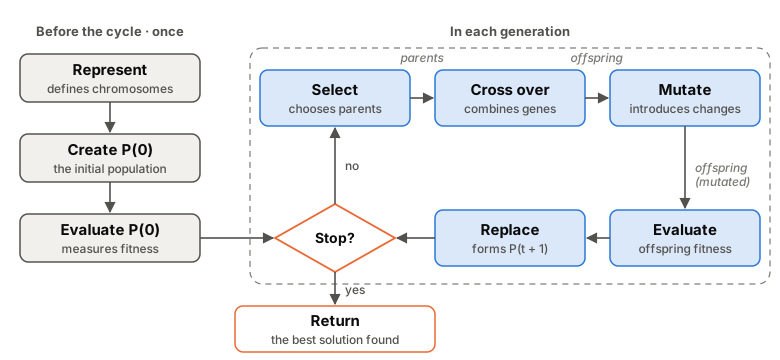
figuras/02-ciclo.py in the book repository.
Two similar-looking decisions must be kept distinct. Selection determines who reproduces; replacement determines who remains in the population. Selection therefore comes at the beginning of a generation, using the current population; replacement comes at the end, once offspring exist.
The figure, pseudocode, and portal use the same order: evaluate the initial population before the cycle, and evaluate offspring after mutation but before replacement. Parent and offspring fitness can then be compared when deciding who remains. With pure generational replacement, offspring could instead be evaluated at the beginning of the next cycle, but we will use one consistent scheme throughout the laboratory.
- Find How they fit into the algorithm and identify the steps under Before the cycle · Once only and In each generation.
- Each step links to the tool explaining it. Which tool do both Select and Replace open? Why do you think they use the same tool?
- Read the final note, beginning “Select chooses the parents.” When must offspring be evaluated before replacement?
These genetic-algorithm steps are out of order: mutate offspring, create the initial population, replace, select parents, represent the problem, evaluate offspring, cross over parents, evaluate the initial population. Put them in order and identify which happen once and which happen every generation.
Show the solution
Once: represent the problem, create the initial population, and evaluate the initial population. Each generation: select parents, cross over parents, mutate offspring, evaluate offspring, and replace. After replacement, check the stopping criterion; if it is not met, begin another generation.2.3 From the Cycle to Pseudocode BasicB
How can we write the cycle so a computer can follow it?
The cycle fits into a few lines of pseudocode, a description independent of any programming language. Let P(t) be the population at generation t, containing N individuals:
 1  t ← 0
 2  P(0) ← create N random individuals
 3  evaluate each individual in P(0)
 4  best ← the fittest individual in P(0)
 5  while the stopping criterion is not met:
 6      parents ← select N parents from P(t)
 7      offspring ← cross over the parents in pairs
 8      offspring ← mutate the offspring
 9      evaluate each offspring; if any is better than best, store it in best
10      P(t + 1) ← replace(P(t), offspring)
11      t ← t + 1
12  return best
Lines 1–4 run once. Lines 6–11 form one generation and repeat until the criterion in line 5 is met. This follows the general evolutionary-algorithm scheme in Talbi (2009, p. 200), with two details worth making explicit.
- Each individual is evaluated once. The initial population is evaluated at line 3; each offspring is evaluated at line 9 as soon as it is created. Evaluation is usually the algorithm’s most expensive operation, so it is not repeated. Section 4.8 returns to this.
- The algorithm remembers the best solution found. The variable best stores the best individual seen so far, even if it later disappears from the population. This is what the algorithm returns (Luke, 2013, algorithm 20).
The names at lines 6, 7, 8, and 10 stand for decisions we have not yet made: how to select (chapter 5), cross over (chapter 6), mutate (chapter 7), and replace (chapter 8). The pseudocode stays the same; what changes between genetic algorithms is what happens inside each line.
With a population of N = 50 individuals and a stopping criterion of 100 generations:
- How many times does line 6 run?
- If each parent pair produces two offspring, how many pairs must be formed per generation? What problem arises if N is odd?
- How many fitness evaluations occur during the whole run?
Show the solution
100 times, once per generation.
Producing 50 offspring requires 25 pairs, N/2. If N were odd, one parent would lack a partner; finding it a partner produces an extra offspring, so one must be discarded (Mitchell, 1996/1998, Section 1.6), or N must be required to be even, as in Luke (2013, algorithm 20).
There are 50 evaluations of the initial population and 50 in each of 100 generations: 50 + 50 \times 100 = 5050. In general, N\,(G + 1) for G generations.
2.4 A Generation by Hand: Represent and Evaluate BasicB
What happens in one generation, number by number?
We will follow a complete generation using a classic example, the “hand simulation” in Goldberg (1989, pp. 15–17). The problem is deliberately simple: find the integer x between 0 and 31 that maximizes
f(x) = x^2 .
The answer is obvious, x = 31, but the algorithm does not know it: it can only propose solutions and ask for their values. We can therefore check whether it moves in the right direction.
Represent. Each solution is written as a 5-bit unsigned binary number, allowing values from 0 (00000) to 31 (11111). The first bit has the greatest weight. For example, 01101 is read as
0 \times 16 + 1 \times 8 + 1 \times 4 + 0 \times 2 + 1 \times 1 = 13 .
Create the initial population. Goldberg takes N = 4 individuals and creates them by tossing a coin 20 times, once per bit (Goldberg, 1989, p. 15): 01101, 11000, 01000, and 10011. We call them A, B, C, and D, as the tool does.
Evaluate. Each individual’s fitness is the function value: decode the string to obtain x, then calculate x^2. For 01101, x = 13 and fitness is 13^2 = 169.
Calculate x and fitness f(x) = x^2 for B = 11000, C = 01000, and D = 10011. What is the sum of all four fitness values? What are the mean and best fitness?
Show the solution
| Individual | Chromosome | x | Fitness x^2 |
|---|---|---|---|
| A | 01101 | 13 | 169 |
| B | 11000 | 24 | 576 |
| C | 01000 | 8 | 64 |
| D | 10011 | 19 | 361 |
2.5 Selecting with the Roulette Wheel BasicB
Given the population’s fitness values, who will become parents?
Goldberg uses roulette-wheel selection: each individual occupies a wheel sector proportional to its fitness, and the wheel is spun as many times as there are parents needed, here four (Goldberg, 1989, pp. 11–12). The probability that a spin selects individual i is its share of total fitness,
p_i = \frac{f_i}{\sum_j f_j} ,
and its expected copies among the N parents are N\,p_i. The same individual can be selected several times. Chapter 5 covers roulette-wheel selection and other mechanisms; this idea is enough here. Think of a draw in which each solution holds as many tickets as its fitness indicates. A fitter solution is more likely to become a parent, but luck still matters: even many tickets may win nothing.
| Individual | A | B | C | D |
|---|---|---|---|---|
| Fitness | 169 | 576 | 64 | 361 |
| Probability p | 0.144 | 0.492 | 0.055 | 0.309 |
| Expected copies, 4 p | 0.58 | 1.97 | 0.22 | 1.23 |
To spin the wheel, the tool draws a random number r between 0 and 1 and places it against the cumulative probabilities: 0.144 for A, 0.637 for A and B together, 0.691 for A through C, and 1 for all four. The first individual whose cumulative probability exceeds r is selected.
Data. The population from exercise 2.4, provided in selection-ga as Goldberg’s example (x²), and the four random numbers from draw 19: r = 0.05, 0.32, 0.45, and 0.75.
Predict. Whom does each spin select? Which individual receives no copies?
Open: roulette with Goldberg’s example
Show the result
The parents are A B B D:
| Spin | 1 | 2 | 3 | 4 |
|---|---|---|---|---|
| r | 0.05 | 0.32 | 0.45 | 0.75 |
| Selected | A | B | B | D |
The number 0.05 is below 0.144 and selects A; 0.32 and 0.45 fall between 0.144 and 0.637, B’s sector; 0.75 falls between 0.691 and 1, D’s sector. C, the worst individual, receives no copies, while B, the best, receives two. Mean fitness rises from 292.5 in the population to 420.5 among the parents.
Goldberg obtained the same outcome with coins: one copy of A, two of B, none of C, and one of D (Goldberg, 1989, p. 16). As he notes, the better individuals receive more copies, the middle ones remain, and the worst disappears. But this is a draw: different r values can produce another result.Show the tool here (roulette with Goldberg’s example)
2.6 Crossover and Mutation BasicB
We have four parents. How do they produce four different offspring?
Form pairs. Goldberg pairs the parents at random; in his simulation, the draw paired the first with the second and the third with the fourth (Goldberg, 1989, p. 16). With parents A B B D, the pairs are A with B (01101 and 11000) and B with D (11000 and 10011). All pairs cross over: crossover probability is 1.
Cross over. Goldberg uses one-point crossover: a cut point is chosen randomly between two genes, and the parents exchange everything to its right (Goldberg, 1989, p. 12). The first offspring takes the first parent’s head and the second parent’s tail; the other does the reverse. In the simulation, for the first pair the cut fell after the fourth gene; for the second pair, after the second (Goldberg, 1989, pp. 16–17, table 1.2). Chapter 6 covers this and other crossover operators.
Data. First pair: Parent 1 0 1 1 0 1 (A) and Parent 2 1 1 0 0 0 (B), cut after gene 4. Second pair: Parent 1 1 1 0 0 0 (B) and Parent 2 1 0 0 1 1 (D), cut after gene 2.
Predict. Write the four offspring. What are their x values and fitness? Is any better than B?
Open: first pair (cut 4) Open: second pair (cut 2)
Show the result
| Pair | Parents | Cut | Offspring | x | Fitness |
|---|---|---|---|---|---|
| 1 | 0110|1 and 1100|0 | 4 | 01100 and 11001 | 12 and 25 | 144 and 625 |
| 2 | 11|000 and 10|011 | 2 | 11011 and 10000 | 27 and 16 | 729 and 256 |
Two offspring outperform B, the best parent (576): 11001 (625) and, especially, 11011 (729). The latter combines B’s beginning, 11, with D’s ending, 11. Neither parent had both its two highest-order bits and its two lowest-order bits set to 1 (Goldberg, 1989, p. 17).
In the first pair, only one gene lies after the cut, so each offspring copies one parent with the other’s final bit. The closer the cut is to the end, the fewer genes are exchanged.Show the tool here (second pair)
Mutate. Finally, each bit in each offspring can flip from 0 to 1 or from 1 to 0 with a small probability, the mutation probability pm. Goldberg uses pm = 0.001 (Goldberg, 1989, pp. 14, 16). With 20 bits in the population, the expected number of mutated bits per generation is 20 \times 0.001 = 0.02: usually no bit mutates, and none did in the simulation. All four offspring remain unchanged. Mutation can restore an allele lost from the population (Goldberg, 1989, p. 14); chapter 7 examines it.
With pm = 0.001 and 20 bits, what is the probability that no bit mutates in a generation? What if pm = 1/5 = 0.2, giving one mutated bit per offspring on average? Hint: if bits are sampled independently, the probability that none changes is the product of their individual probabilities of not changing.
Show the solution
Each bit stays unchanged with probability 1 - \mathit{pm}, and all 20 bits are sampled independently. The probability of no mutation is (1 - 0.001)^{20} = 0.999^{20} \approx 0.980. With pm = 0.2, it is 0.8^{20} \approx 0.012: at least one mutation is almost certain, and on average 20 \times 0.2 = 4 bits mutate, one per offspring.- The link opens bit-flip mutation with offspring 1 1 0 1 1. Advance step by step: a number r is drawn at each position, and the bit changes if r is below pm.
- Set pm to its minimum, 0.01, and click Draw again several times. How often does any bit change? The tool does not go below 0.01, so Goldberg’s 0.001 cannot be entered; at that value, changes would be ten times rarer still.
- Set pm = 0.2 and repeat. How many bits change in each draw?
2.7 Replace and Compare BasicB
We have four offspring. Is the new population better than the old one?
In Goldberg’s algorithm, offspring replace every parent: generational replacement, as in the canonical genetic algorithm (Talbi, 2009, pp. 202, 221). The new population is decoded and evaluated, completing the generation.
Data. The initial parents A–D, with fitness values 169, 576, 64, and 361, and the four offspring from example 2.6, named a–d in the tool: a = 01100 (144), b = 11001 (625), c = 11011 (729), and d = 10000 (256). The screen is called “Generational with elitism”; setting Elite size e to 0 gives pure generational replacement.
Predict. Who forms the generation 1 population? How do mean and best fitness change?
Open: generational replacement, e = 0
Show the result
Generation 1 is a b c d: all four offspring enter, and no parent remains.
| Generation 0 | Generation 1 | |
|---|---|---|
| Population | 01101, 11000, 01000, 10011 | 01100, 11001, 11011, 10000 |
| Sum of fitness values | 1170 | 1754 |
| Mean fitness | 292.5 | 438.5 |
| Best fitness | 576 (x = 24) | 729 (x = 27) |
Show the tool here (generational replacement)
Why did the population improve? Selection gave two copies to B, the best, and none to C, the worst. In 11011, crossover combined B’s useful beginning, 11, with D’s useful ending, 11 (Goldberg, 1989, p. 17). Together, selection and crossover combine parts of good solutions to produce better ones.
One generation of a random process is not enough to draw general conclusions, however (Goldberg, 1989, p. 16). Other random numbers might have selected C or caused crossover to break up B’s useful structure. Nothing guarantees that the new population retains its best individual, as the next exercise shows.
Another classic example (Mitchell, 1996/1998, Section 1.6) uses 8-bit strings whose fitness is their number of ones. Initial fitness values are A = 2, B = 6, C = 1, and D = 3. After selection, crossover with probability 0.7 (one of the two pairs did not cross over), and mutation, offspring fitness values are 3, 5, 1, and 5. Under generational replacement, what happens to mean and best fitness? What changes if the best parent enters the next generation instead of the worst offspring?
Show the solution
The mean rises from 12/4 = 3 to 14/4 = 3.5, but best fitness falls from 6 to 5: B, the best individual, is lost. If B replaces the worst offspring, whose fitness is 1, the next generation has values 6, 3, 5, and 5: best fitness stays at 6 and the mean rises to 4.75. This is elitism, covered in section 8.3. Check both cases in selection-ga: without an elite and with one elite individual. The tool rounds the mean to 4.8.2.8 Nine Design Decisions BasicB
Someone chose 5 bits, roulette-wheel selection, one-point crossover, and the other settings for Goldberg’s problem. What must be decided when building a genetic algorithm in general?
Each box in figure 2.1 contains one or more decisions. Talbi (2009, p. 205) groups them into seven components: representation, population initialization, objective function, selection, reproduction (crossover and mutation), replacement, and stopping criterion. Separating crossover from mutation and decoding from representation gives nine design decisions:
| Decision | Question | In Goldberg’s example | Chapter |
|---|---|---|---|
| 1. Representation | How is a solution written as a chromosome? | A 5-bit string | 3 |
| 2. Initialization | What population starts the search? | 4 random strings | 4 |
| 3. Genotype and phenotype | How does a chromosome become a solution? | Unsigned binary to an integer from 0 to 31 | 3 |
| 4. Fitness | How is solution quality measured? | f(x) = x^2 | 4 |
| 5. Mutation | How are small changes introduced? | Bit-flip mutation, pm = 0.001 | 7 |
| 6. Crossover | How are two parents combined? | One-point, always | 6 |
| 7. Selection | Who reproduces? | Roulette wheel | 5 |
| 8. Replacement | Who enters the next generation? | Generational: all offspring | 8 |
| 9. Stopping | When does the run end? | After one generation, for the example | 8 |
We also choose parameter values, such as population size N and crossover and mutation probabilities, discussed in chapter 9.
The table follows design order, not execution order. Representation comes first because other decisions depend on it: fitness is calculated from the decoded solution, while crossover and mutation act on the chromosome (Talbi, 2009, p. 200), so they must suit its form. One-point crossover, for example, works with bit strings but not with a traveling-salesman route written as a permutation, because offspring may repeat cities (section 6.5). Selection and replacement, by contrast, use only fitness and therefore work with any representation.
A team designs a genetic algorithm for the traveling salesman problem: a delivery driver leaves a depot, visits every customer once, and returns to the depot; the aim is the shortest route (section 10.2 develops the full problem). Which of the nine decisions does each statement describe?
- “Each route will be a permutation of customers.”
- “Fitness will be the inverse of route length.”
- “To obtain the route, add the depot at the beginning and end of the permutation.”
- “The two best individuals will enter the next generation unchanged.”
- “Stop after 100 generations without improvement.”
- “With probability 0.05, exchange two customers in an offspring.”
- “Choose parents by tournament among 4 individuals.”
Show the solution
a) Representation (1). b) Fitness (4). c) Genotype and phenotype (3): the permutation is the chromosome, and the complete route is the solution. d) Replacement (8): elitism. e) Stopping (9). f) Mutation (5). g) Selection (7).2.9 From a Generation to a Run BasicB
One generation improved Goldberg’s population. What happens if the cycle continues?
A genetic algorithm does not stop after one generation: it repeats the cycle tens or hundreds of times. The sequence from the initial population to stopping is a run (Mitchell, 1996/1998, Section 1.6). The stopping criterion may be fixed in advance, such as a number of generations or evaluations, or depend on events during the run, such as several generations without improvement or a sufficiently good solution (Talbi, 2009, pp. 198–199). Section 8.6 examines this.
Since most steps use random numbers, two runs with different seeds usually end at different points (Mitchell, 1996/1998, Section 1.6). Understanding an algorithm’s behavior therefore requires several runs, as discussed in chapter 9.
EvoTraveller shows a complete run. It solves the traveling salesman problem from exercise 2.8: the depot is the origin, at (0, 0), and the customers are locations on a grid. Each individual is a permutation of locations, and its fitness is the inverse of route length: higher fitness means a shorter route.
- If Zzzz appears, click Yes, get this app back up! and wait for the controls to appear.
- Enter the sidebar reference settings and click Run. Fitness shows each generation’s best fitness, from 0 to 50; Best solution shows the final best route.
- Under Solutions, move Generation from 0 onward and watch the population’s routes change. Are they more alike at the beginning or at the end?
- Under GA parameters in the sidebar, identify the controls for selection, crossover, mutation, replacement, and stopping. Which design decisions cannot be changed?
- Set Generations to 10 and click Run again. Which decision changed? Does the curve reach the same value as with 50? At which generation does it stop improving? Section 9.1 returns to this.
According to its description and code, EvoTraveller initializes with random permutations, selects parents by tournament, crosses them with OX, mutates by exchanging two locations, and passes the best individuals into the next generation unchanged. To form a route, it adds the origin to the beginning and end of the permutation.
- Complete the table from section 2.8 for EvoTraveller and identify the corresponding sidebar control, if one exists.
- With the reference settings, the Fitness curve rises or stays level, but never falls. Why?
Show the solution
- The completed table:
| Decision | In EvoTraveller | Control |
|---|---|---|
| 1. Representation | A permutation of locations | — |
| 2. Initialization | Random permutations | Population size sets how many |
| 3. Genotype and phenotype | Add the origin at the beginning and end | — |
| 4. Fitness | Inverse of route length | — |
| 5. Mutation | Exchange two locations | Mutation rate |
| 6. Crossover | OX | Crossover |
| 7. Selection | Tournament | Tournament size |
| 8. Replacement | Generational with an elite | Elitism |
| 9. Stopping | A fixed number of generations | Generations |
Number of places sets problem size. Seed fixes both location positions and the algorithm’s random draws, making the map and run reproducible. Changing it changes both, as section 9.1 explains.
- Because there is an elite: the best individuals enter the next generation without crossover or mutation, so one generation’s best route remains in the next. Best fitness can only rise or remain unchanged, as in exercise 2.7 with an elite.
Summary
- A genetic algorithm evolves a population of solutions. Representing the problem, creating the initial population, and evaluating it happen once; selection, crossover, mutation, offspring evaluation, and replacement repeat each generation until the stopping criterion is met.
- Selection determines who reproduces; replacement determines who remains. Each individual is evaluated once, and the algorithm returns the best solution found.
- In Goldberg’s generation, roulette-wheel selection gives fitter individuals more copies, and crossover combines useful parts from two parents: mean fitness rises from 292.5 to 438.5 and best fitness from 576 to 729. But a generation is a random outcome, and without an elite the best can be lost.
- Designing a genetic algorithm requires nine decisions: representation, initialization, genotype and phenotype (decoding), fitness, mutation, crossover, selection, replacement, and stopping. Representation comes first because it constrains fitness and the operators.
To continue along the basic path, go to “Representing Solutions”.
2.10 Variants of the Cycle AdvancedA
Do all genetic algorithms follow exactly the same cycle?
The cycle in figure 2.1 is the most common, but some variants change important details.
- Not every pair crosses over. Goldberg’s example uses crossover probability 1. Usually it is lower, for example 0.7: with that probability the pair crosses over; otherwise its offspring copy the parents and can then mutate (Mitchell, 1996/1998, Section 1.6). In exercise 2.7, one pair did not cross over.
- Forming pairs. Goldberg pairs parents randomly after selecting them all (Goldberg, 1989, p. 16); other algorithms select each pair directly, one parent at a time (Mitchell, 1996/1998, Section 1.6; Luke, 2013, algorithm 20). When selection chooses parents independently, the result is the same.
- Where evaluation happens. The scheme in Talbi (2009, p. 200) evaluates the population at each generation’s beginning and also evaluates offspring before replacement. Taken literally, this evaluates each offspring twice: when created and when the next generation begins. A careful implementation stores each individual’s fitness instead of recalculating it (section 4.8).
- Generational or steady-state. Generational replacement creates N offspring per generation to replace the whole population. A steady-state algorithm creates one offspring, or a few, to replace, for example, the population’s worst individual (Talbi, 2009, p. 221). A “generation” is then much shorter, so comparing algorithms requires counting evaluations rather than generations (section 8.4).
- Remembering the best solution. The pseudocode variable best stores the best solution found outside the population (Luke, 2013, algorithm 20). Elitism retains it inside the population, where it can also continue reproducing (section 8.3).
A generational algorithm with N = 50 runs for 100 generations. A steady-state algorithm, also with N = 50, creates one offspring per step. How many evaluations does the first perform? How many steps does the second need for the same total? If the first literally followed Talbi’s scheme without storing fitness, how many evaluations would it perform?
Show the solution
The generational algorithm evaluates the 50 initial individuals and 50 offspring per generation: 50 + 50 \times 100 = 5050 evaluations. The steady-state algorithm evaluates the 50 initial individuals and one offspring per step, so it needs 5000 steps to reach the same 5050. Without stored fitness, Talbi’s scheme evaluates the population (50) and offspring (50) every generation: 100 evaluations each, or 10 000 over 100 generations, almost twice as many. The extra 4950 repeat existing calculations: from the second generation onward, the population evaluated at the beginning consists of offspring already evaluated in the previous generation.2.11 Further Reading Further reading+
A family of algorithms. Genetic algorithms are evolutionary algorithms, which are themselves population-based metaheuristics. All follow the same scheme: generate a new population and select which population to keep (Talbi, 2009, p. 191). Representation and operators distinguish the families. Holland’s genetic algorithms characteristically use binary strings, n-point or uniform crossover, bit-flip mutation, fitness-proportionate selection, and generational replacement. Evolution strategies (Rechenberg and Schwefel) use real-valued vectors, Gaussian mutation, and (μ, λ) or (μ + λ) replacement. Evolutionary programming (Fogel) does not use crossover, while genetic programming (Koza) evolves programs represented as trees (Talbi, 2009, pp. 201–204, tables 3.4 and 3.5). Today the boundaries are blurred: some genetic algorithms use nonbinary representations (Talbi, 2009, p. 201), and real-vector algorithms such as those in chapter 6 borrow ideas from evolution strategies.
Why does it work? In example 2.6, the best offspring combined two parts of good strings: 11 at the beginning and 11 at the end. Goldberg (1989, p. 17) uses this observation to analyze genetic algorithms through schemata, or similarity templates: a pattern such as 11*** describes every string beginning with 11. This is where classical theoretical analysis of genetic algorithms begins (Goldberg, 1989, p. 1); we do not need it to use them.
More to read. The full hand simulation, with more detail about each operator, appears in Goldberg (1989, pp. 10–17). Mitchell (1996/1998, Section 1.6) describes the same algorithm as a list of steps with another example. Talbi (2009, Sections 3.1–3.3) presents the shared evolutionary-algorithm scheme and its components, while Luke (2013, algorithm 20) gives genetic-algorithm pseudocode close to section 2.3.