10 The Traveling Salesman from Start to Finish
Tools: EvoTraveller, crossover-ga, and mutation-ga, available through the portal. EvoTraveller has an English-only interface.
After completing the basic path through this chapter, you will be able to:
- describe the traveling salesman problem, its representation with permutations, and its fitness, and calculate the length of a route;
- apply by hand a complete generation to a population of routes: evaluate, select, cross over, mutate, and replace;
- interpret what EvoTraveller shows during a run: the fitness curve, the best route, and the population’s loss of diversity;
- explain what the elite does in replacement and why its size matters less than its existence;
- choose EvoTraveller’s parameters with maps similar to the real case and estimate the quality of the choice with maps that were not used to make it.
10.1 First, Observe BasicB
What does a genetic algorithm do with a routing problem, from the first generation to the last?
In the previous chapters we studied each piece separately: representation, the initial population and fitness, selection, crossover, mutation, replacement, and parameters. In this chapter we put them together in a single problem, the traveling salesman problem, with EvoTraveller (Santos et al., 2025). We already used it in section 2.9 and in chapter 9. Before explaining anything, we will watch an entire run and note down what we see. The explanations will come in the following sections.
This table summarizes which pieces reappear, where they were studied, and where you will find them here. If you do not remember one of them, it is a good idea to review it first:
| Piece | Where it was studied | Where it reappears |
|---|---|---|
| Permutation | Section 3.5 | Section 10.2 |
| Fitness from a cost: the inverse | Section 4.6 | Section 10.2 |
| Tournament | Section 5.2 | Section 10.3 |
| OX crossover and its variants | Sections 6.6 and 6.9 | Section 10.3 |
| Swap mutation | Section 7.6 | Section 10.3 |
| Elite | Section 8.3 | Sections 10.3 and 10.5 |
| Premature convergence | Section 9.7 | Section 10.4 |
| Replicates and similar cases | Sections 9.3 and 9.5 | Section 10.6 |
| Horizon and budget | Section 9.6 | Section 10.6 |
EvoTraveller has three charts. Fitness shows the fitness of the best route in each generation; fitness is the inverse of length, so if it rises, the best route is shorter. Best solution draws the best route at the end. And under Solutions, the Generation control chooses a generation, and the chart draws all the routes in the population in that generation, each in its own cell.
Data. In EvoTraveller, keep the reference values in the sidebar: Number of places 10, Seed 1111, Population size 100, Generations 50, Tournament size 4, Mutation rate 0.05, Elitism 0.05, and Crossover 0.6. Click Run. Then, under Solutions, move Generation to 0, to 10, and to 49, the last value.
Predict. Does the Fitness curve keep rising until generation 50? Are the routes in the population similar to one another at the beginning? And at the end?
Open and configure: EvoTraveller
Show the result
- The curve rises at first and then stays flat. Fitness goes from 0.0230 in generation 0 to 0.0293 in generation 3, and it does not change during the next 47 generations. The best route has length 34.11, the inverse of 0.02932.
- In generation 0, the 100 chromosomes are all different (99 routes: two are the same route traveled in reverse), and almost all of them are very tangled.
- In generation 10, there are many repeated routes. Only 30 distinct routes remain, and 43 of the 100 drawings are the same route: the best one, of length 34.11.
- In generation 49, the best route is still the same. There are 23 distinct routes, and 46 drawings are the best route. The others are variations of it, some of them considerably worse.
With what you have seen in example 10.1, write down a provisional answer to each question. We will answer them in the following sections.
- Why does the Fitness curve never go down, not even a little?
- Why does the population fill up with copies of the same route?
- The best possible route on this map has length 31.50 (section 9.1). Why does the algorithm stop improving in generation 3 if it still has 47 generations left?
Show the solution
You already saw it in exercise 2.9: because of the elite, the best routes pass unchanged into the next generation. We will see this in section 10.5.
Because the elite and the copies of tournament winners, which are almost always the best route, take up a large part of the population, and mutation changes only 5% of the individuals. We will calculate this in exercise 10.4.
Because the population has lost diversity: almost everything that is crossed over consists of copies of the same route or small variations of it, and nothing better appears. This is the premature convergence of section 9.7. We will see this in section 10.4.
10.2 The Problem and Its Representation BasicB
How is a route turned into a chromosome, and how many routes are there?
The traveling salesman problem is probably the most popular combinatorial optimization problem. Given n cities and the distance between each pair, we must find the shortest tour that visits each city exactly once and returns to the starting point (Talbi, 2009, p. 7). It is easy to state and very hard to solve, and because so much is known about it, it is used as a test bed: new combinatorial optimization methods are usually tried on the traveling salesman problem to get an idea of how useful they are (Larrañaga et al., 1999, p. 132). In EvoTraveller, the starting point is an origin O at position (0, 0), and the other places are at integer points on a 10 × 10 grid. The distance between two places is the straight-line distance, and the length of a route is the sum of the distances of its legs.
Representation. A tour is an order of visits, so the natural representation is a permutation of the places, as in section 3.5: each place appears exactly once (Talbi, 2009, p. 36). It is also the representation most used in genetic algorithms for the traveling salesman problem (Larrañaga et al., 1999, p. 134); there are others, which you will see in section 10.9. The origin is not part of the chromosome, because it is always first and last. The chromosome is the genotype; the complete route, with the origin at the beginning and at the end, is the phenotype (section 3.1). In this chapter, we write the chromosome with the numbers of the places: 3 4 1 2 5 is the route O → 3 → 4 → 1 → 2 → 5 → O.
Fitness. We want to minimize the length L, and EvoTraveller uses its inverse as fitness, f = 1/L, which is larger the shorter the route is (section 4.6). Because EvoTraveller’s selection is a tournament, which only looks at which route is better than another, choosing the shorter route directly would give the same result.
Size of the search space. With n places counting the origin, there are (n-1)! different chromosomes. But a route and the same route traveled in reverse have the same length: 3 4 1 2 5 and 5 2 1 4 3 are the same tour. The distinct routes are half as many:
| Places (n) | Chromosomes, (n-1)! | Distinct routes, (n-1)!/2 |
|---|---|---|
| 6 | 120 | 60 |
| 10 | 362 880 | 181 440 |
| 15 | 87 178 291 200 | 43 589 145 600 |
Each additional place multiplies the number of routes by the number of places there already were: going from 10 to 11, by 10. With 15 places there are more than 40 billion, which is why they cannot all be checked except on small maps.
To work by hand, we will use a small EvoTraveller map with the usual seed: Number of places 6 and Seed 1111. That is the origin and five places (figure 10.1).
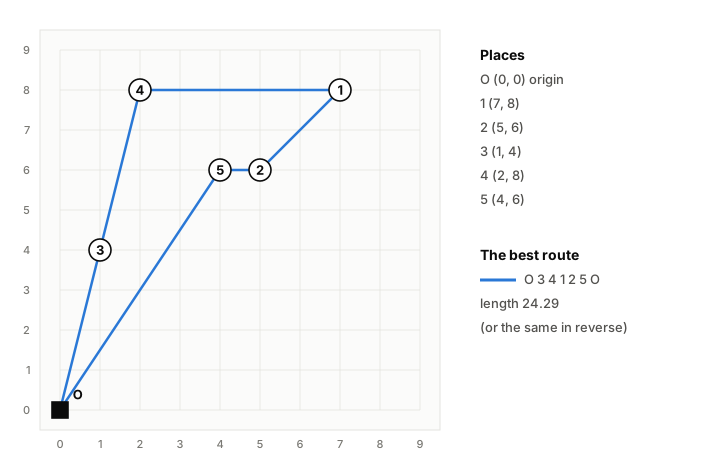
figuras/10-viajante.py in the book’s repository.
Distances between the places, rounded to two decimal places:
| O | 1 | 2 | 3 | 4 | 5 | |
|---|---|---|---|---|---|---|
| O | — | 10.63 | 7.81 | 4.12 | 8.25 | 7.21 |
| 1 | 10.63 | — | 2.83 | 7.21 | 5.00 | 3.61 |
| 2 | 7.81 | 2.83 | — | 4.47 | 3.61 | 1.00 |
| 3 | 4.12 | 7.21 | 4.47 | — | 4.12 | 3.61 |
| 4 | 8.25 | 5.00 | 3.61 | 4.12 | — | 2.83 |
| 5 | 7.21 | 3.61 | 1.00 | 3.61 | 2.83 | — |
The route lengths in this chapter are calculated with the unrounded distances. If you add up those in the table, you will sometimes get a difference of one hundredth.
Data. In EvoTraveller, set Number of places to 6 and keep the other reference values (Seed 1111, Population size 100, Generations 50). Click Run. Then set Population size to 10 and Generations to 10, and click Run again.
Predict. With 100 individuals, how many generations will the algorithm need to find the route in figure 10.1? And with 10?
Open and configure: EvoTraveller
Show the result
With 100 individuals, none: the Fitness curve is flat from generation 0, at 0.0412, which is 1/24.29. There are only 120 possible chromosomes, and it is likely (about 81%) that an initial population of 100 random chromosomes contains one of the two that give the best route; in this run, it does. Best solution draws the route O 3 4 1 2 5 O.
With 10 individuals, nine generations. The best fitness starts at 0.0384 (length 26.01), rises to 0.0390 (25.66) in generation 1 and to 0.0403 (24.80) in generation 8, and reaches 0.0412 (24.29) in generation 9.
With such a small problem, the genetic algorithm is not needed: it is enough to check the 60 routes. We use it because it can be followed by hand.- Using the distance table, calculate the length of route 3 1 2 4 5.
- Write the chromosome of the same route traveled in reverse. Why does it have the same length?
- Why is a vector of five integers from 1 to 5, chosen freely, not suitable as a chromosome?
Show the solution
The route is O → 3 → 1 → 2 → 4 → 5 → O. The lengths of its legs add up to 4.12 + 7.21 + 2.83 + 3.61 + 2.83 + 7.21 = 27.81.
In reverse, the route is O → 5 → 4 → 2 → 1 → 3 → O, with chromosome 5 4 2 1 3. It uses the same six legs, traveled in the opposite direction, and the distance between two places is the same in both directions.
Because a vector of integers can repeat places and leave others unvisited, for example 3 1 3 4 5, which passes through 3 twice and never through 2. It would not be a valid tour. A permutation guarantees that each place appears exactly once (section 3.5).
10.3 One Generation by Hand BasicB
What happens to a population of routes in one generation?
We will carry out by hand a generation like those in EvoTraveller, with a population of only four routes on the map in figure 10.1. Each EvoTraveller generation has three parts: the elite, which is carried over unchanged; copies of selected individuals, which may mutate; and offspring of pairs of selected individuals, which are crossed over and may mutate. With four individuals, we will take one elite individual (EvoTraveller would round it up to 2; here we use 1 to keep things simple), one copy, and one pair, which gives two children. Selection is a tournament of two; crossover is EvoTraveller’s OX; and mutation is a swap of two places, with pm = 0.2 per individual, the highest value the tool allows.
The draws are fixed in advance. We chose them so that all the cases we want to see appear in a single generation.
1. Evaluate. The initial population has four randomly drawn routes:
| Individual | Chromosome | Length L | Fitness 1/L |
|---|---|---|---|
| A | 5 2 1 3 4 | 30.62 | 0.0327 |
| B | 3 1 2 4 5 | 27.81 | 0.0360 |
| C | 2 1 3 5 4 | 32.53 | 0.0307 |
| D | 1 5 4 2 3 | 29.26 | 0.0342 |
The mean length is 30.06, and the best route is B.
2. Elite. The best route, B, passes unchanged into the next generation (section 8.3).
3. Select. Three tournaments are played between two distinct individuals, and the one with the shorter route wins (section 5.2):
| Tournament | Contestants | Winner | Destination |
|---|---|---|---|
| 1 | B and C | B | Parent 1 |
| 2 | A and C | A | Parent 2 |
| 3 | D and A | D | Copy |
C, the worst route, does not win any tournament. With two distinct contestants, the worst can never win.
4. Cross over. EvoTraveller crosses with OX in the variant that crossover-ga calls “Order from the start”, which is not the classic one from section 6.6, but the one from section 6.9. The cuts fall after the first gene and after the third, so the segment is positions 2–3. To form Child 1:
- copy the segment of Parent 1 (B): · 1 2 · ·;
- read Parent 2 (A) from the first position, skipping the places already present: from 5 2 1 3 4, this leaves 5, 3, and 4;
- fill the gaps in that order starting after the second cut: positions 4 and 5 and then, wrapping around, position 1.
Child 1 is 4 1 2 5 3. Child 2 is formed in the same way, with the roles swapped: it takes the segment from A, · 2 1 · ·, and from B, read from the beginning, 3, 4, and 5 remain. Child 2 is 5 2 1 3 4, the same as A.
5. Mutate. Each new individual, except the elite, mutates with probability pm = 0.2. A number is drawn for each one: 0.71 for the copy of D, 0.48 for Child 1, and 0.13 for Child 2. Only the last is less than 0.2, so only Child 2 mutates. The swap draws two positions, 4 and 5, and exchanges them: 5 2 1 3 4 becomes 5 2 1 4 3.
Data. OX crossover in the “Order from the start” variant, with Parent 1 = 3 1 2 4 5 (B), Parent 2 = 5 2 1 3 4 (A), and the segment at positions 2–3. Then, swap mutation of Child 2, 5 2 1 3 4, at positions 4 and 5.
Predict. What are the lengths of the two children and of the mutant? Does any of them improve on B, the best route in the population?
Open: OX crossover as in EvoTraveller Open: swap mutation of Child 2
Show the result
| Individual | Chromosome | Length |
|---|---|---|
| Child 1 | 4 1 2 5 3 | 24.80 |
| Child 2 | 5 2 1 3 4 | 30.62 |
| Mutated Child 2 | 5 2 1 4 3 | 24.29 |
Show the tool here (OX crossover, “Order from the start”)
6. Replace. The next generation consists of the elite, the copy, and the two children (figure 10.2):
| Individual | Origin | Chromosome | Length |
|---|---|---|---|
| B | Elite | 3 1 2 4 5 | 27.81 |
| D | Copy, not mutated | 1 5 4 2 3 | 29.26 |
| H1 | Child 1, not mutated | 4 1 2 5 3 | 24.80 |
| H2 | Child 2, mutated | 5 2 1 4 3 | 24.29 |
The mean length falls from 30.06 to 26.54, and the best route from 27.81 to 24.29. C has disappeared, and all that remains of A is what has passed to the children.
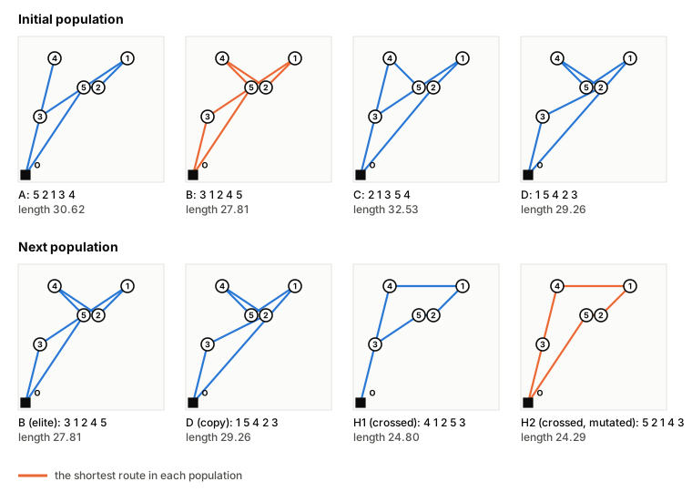
figuras/10-viajante.py in the book’s repository.
With five destinations and the origin, there are only 60 routes, and it is easy to hit on the best one. On a map of 15 places, with more than 40 billion routes, a single generation achieves much less: improvement is slow and depends on many generations.
Repeat step 4 with the classic OX from section 6.6, which reads the other parent starting after the second cut. With the same parents, the same segment, and the same mutation of Child 2 at positions 4 and 5, which children come out, and what is the best route in the next generation?
Show the solution
Child 1: the segment from B is · 1 2 · ·. A, read starting after the second cut, is 3 4 5 2 1; without 1 and 2, this leaves 3, 4, and 5, which go to positions 4, 5, and 1. Child 1 is 5 1 2 3 4, of length 30.49.
Child 2: the segment from A is · 2 1 · ·. B, read starting after the second cut, is 4 5 3 1 2; 4, 5, and 3 remain. Child 2 is 3 2 1 4 5, of length 26.46. Mutated at positions 4 and 5, it becomes 3 2 1 5 4, of length 26.10.
The next generation would be B (27.81), D (29.26), 5 1 2 3 4 (30.49), and 3 2 1 5 4 (26.10). The best route would be 3 2 1 5 4, which improves on B but does not reach 24.29. With the same draws, the crossover variant changes the children. Both variants preserve the segment of one parent and the relative order of the other, and neither is better in general; in the traveling salesman problem, what matters are the legs (section 9.10).- The tool opens with parents B and A and the “Order from the start” Variant, EvoTraveller’s. Drag the cuts to try other segments and note down the children. With this variant, no segment gives the best route, 3 4 1 2 5 or 5 2 1 4 3.
- Change the Variant to “Classic (Goldberg, 1989)” and try segments again. With which one does Child 2 give the best route?
10.4 What Happened in the Run BasicB
With what we have done by hand, how can we explain what we saw in the run in example 10.1?
The curve never goes down because there is an elite: the best route in one generation passes unchanged into the next, like B in section 10.3. The best fitness can only rise or stay the same.
The population fills up with copies because several pieces push in the same direction. The elite already consists of 6 copies of the best route. The tournament favors the best routes, and the more copies of the best route there are, the more tournaments it wins. An unmutated copy is identical to its parent, and with Mutation rate 0.05, only one individual in twenty mutates. In generation 10, 43 of the 100 individuals were the best route.
The algorithm stops improving because it has lost diversity. Almost half the population is the same route, and many crossovers are between two copies of it. With EvoTraveller’s OX, which is not pure, because two identical parents do not always give an identical child (example 6.11), crossing two copies gives the same route only if the segment starts at the first position; otherwise, it gives the same route with a piece shifted. On this map, none of those children is shorter than the best route: of the 36 possible pairs of cuts, 8 repeat it and 28 make it longer. And what mutation brings is not enough to find a better route. The search gets stuck around a route of 34.11, while the best possible one measures 31.50: this is the premature convergence of section 9.7. The population keeps changing, but nothing better appears.
Selection pressure (chapter 5) determines how fast diversity is lost. In EvoTraveller it is controlled by Tournament size.
Data. EvoTraveller’s reference values, except Tournament size, which takes two values: 2 and 10. Click Run with each one and look at the population with Generation 10.
Predict. With which tournament are there more copies of the best route in generation 10?
Open and configure: EvoTraveller
Show the result
| Tournament size | Distinct routes in generation 10 | Copies of the best route | Length of the best route |
|---|---|---|---|
| 2 | 73 | 14 | 31.86 |
| 4 (initial value) | 30 | 43 | 34.11 |
| 10 | 22 | 57 | 31.50 |
With the tournament of 10, more than half the population consists of copies of the best route; with the tournament of 2, only 14. The larger the tournament, the higher the selection pressure and the faster diversity is lost.
Look at the last column: on this map, the tournament of 10 finds the best possible route and the tournament of 4 does not. But this is a single run on a single map, and we already know that this is not enough (section 9.3).To find out what happens in general, we repeated the experiment with 30 maps of 10 places, those of seeds 1111 to 1140, with one run on each map. A separate program gives us the best route on each map, and we count on how many of them EvoTraveller finds it:
| Configuration | Distinct routes in generation 10 (mean) | Maps on which it finds the best route |
|---|---|---|
| Tournament of 2 | 72.8 | 29 of 30 |
| Tournament of 4 (reference values) | 43.3 | 17 of 30 |
| Tournament of 10 | 22.0 | 13 of 30 |
| Tournament of 4 with Mutation rate 0.2 | 58.9 | 28 of 30 |
With more selection pressure, fewer distinct routes are kept and the algorithm gets stuck more often. Mutating more also preserves diversity. EvoTraveller’s reference values are not the best for these maps.
In generation 10 of example 10.1, 43 of the 100 individuals are the best route. With the reference values, each EvoTraveller generation has 6 elite routes, 34 copies of tournament winners, and 60 crossover offspring (we will see this in section 10.7). Each tournament pits 4 distinct individuals against one another, and each copy or child mutates with probability 0.05.
- What is the probability that a copy of the best route wins a tournament?
- How many of the 34 copies will be, on average, the unmutated best route?
- Crossing two copies of the best route repeats it only if the segment starts at the first position, which happens in 2 of every 9 draws of cuts with 9 places. How many of the 60 children will be, on average, the best route? How many copies do you expect in total?
Show the solution
There are 57 individuals that are not the best route. The probability that all 4 contestants are drawn from them is
\frac{57}{100} \cdot \frac{56}{99} \cdot \frac{55}{98} \cdot \frac{54}{97} \approx 0.10.
If there is at least one copy of the best route in the tournament, it wins, so the probability is 1 - 0.10 = 0.90.
Each copy is the best route with probability 0.90 and does not mutate with probability 0.95: on average, 34 \times 0.90 \times 0.95 \approx 29.
Both parents are the best route with probability 0.90^2 \approx 0.81. On average, 60 \times 0.81 \times \frac{2}{9} \times 0.95 \approx 10 children. In total, 6 + 29 + 10 = 45 copies, very close to the 43 observed. Most come from the elite and the copies, not from crossover.
10.5 The Elite in Replacement BasicB
How many of the best routes should be kept from one generation to the next?
EvoTraveller uses generational replacement with an elite (section 8.3): the e best routes pass unchanged, and the rest of the population is replaced by copies and offspring. The size of the elite is set by Elitism, as a fraction of the population. With the reference values, Elitism 0.05 and 100 individuals, the elite consists of 6 routes (in section 10.7 we will see why 6 and not 5).
But the elite is the first 6 positions of the sorted population, not 6 distinct routes. In example 10.1, from generation 5 onward, the 6 positions are occupied by copies of the same route, because the best one already has many copies. An elite of 6 then keeps the same as an elite of 1.
Data. EvoTraveller’s reference values, except Elitism, which takes three values: 0.01, 0.05, and 0.1. Click Run with each one.
Predict. With which elite is the shortest route found?
Open and configure: EvoTraveller
Show the result
| Elitism | Elite routes | Final fitness | Final length |
|---|---|---|---|
| 0.01 | 2 | 0.0317 | 31.50 |
| 0.05 | 6 | 0.0293 | 34.11 |
| 0.1 | 10 | 0.0317 | 31.50 |
With the 30 maps of 10 places from section 10.4, one run per map, the number of maps on which the best route is found is:
| Mutation rate | Elitism 0.01 | Elitism 0.05 | Elitism 0.1 |
|---|---|---|---|
| 0.05 | 26 | 17 | 20 |
| 0.2 | 23 | 28 | 27 |
There is no clear order: with little mutation the small elite wins, and with more mutation the intermediate one. The differences change direction when another parameter changes. This is what we would expect if the elite almost always keeps the same route, the best one, whatever its size.
What does matter is that there is an elite. EvoTraveller does not let you disable it, but we can do so by changing one line of its code, and repeat the experiment with 30 maps of 15 places (seeds 1111 to 1140) and pm = 0.2:
| Replacement | Mean gap above the best route | The best-route curve gets worse at some point | The final route is worse than the best found |
|---|---|---|---|
| With an elite (6 routes) | 6.1% | 0 of 30 | 0 of 30 |
| Without an elite | 10.2% | 28 of 30 | 13 of 30 |
Without an elite, the best route in a generation can be lost: if it mutates or is crossed over, its offspring may be worse. In 13 of the 30 runs, the route the algorithm delivers at the end is worse than another it had found earlier. With pm = 0.05 the difference is much smaller (13.7% with an elite and 13.5% without one), because the copies of the best route almost never mutate. The elite makes heavy mutation cheap, as seen in section 9.9.
Repeat the replacement from section 10.3 without an elite. Instead of B, a second copy enters the next generation: that of the winner of a fourth tournament between B and D, which does not mutate. a) What is the next generation, and what is its best route? b) Now imagine that the fourth tournament is played by C and D, Child 2 does not mutate, and Child 1 turns out worse than B. What happens to the best route?
Show the solution
B wins the tournament against D, so the next generation would be the same: B (as a copy), D, and the two children, H1 and H2. Its best route is that of H2, with length 24.29. Here the elite changes nothing, because the tournament has already chosen B.
D wins the fourth tournament against C. D enters twice, along with Child 1 and the unmutated Child 2 (5 2 1 3 4, with length 30.62). No route reaches 27.81: the best route in the next generation is worse than B, and the best-fitness curve goes down. The elite guarantees that this does not happen.
10.6 From Trial to Real Case BasicB
Every week, a company delivers from its warehouse to 14 customers, whose positions change from one week to the next. How do we choose EvoTraveller’s parameters to calculate their routes?
It is a tactical problem (section 9.6): it is solved every week, the quality of the route matters, and there is limited time to calculate it. Suppose the time allows about 5000 route evaluations per week, those of EvoTraveller’s reference values: 100 routes in each of the 51 generations, from 0 to 50. We are going to bring together everything we have seen in chapter 9 and in this one.
1. Cases similar to the real one. We do not know the maps for the coming weeks, but we do know what they are like: 15 places counting the warehouse. We will use EvoTraveller maps of that size (section 9.5).
2. A measure. On each map, how much longer the algorithm’s route is than the best possible one, as a percentage. Here the best route is calculated by an exact program; in a real case, it would be compared with the best known route.
3. Three groups of maps. We tune with 10 maps (seeds 1111 to 1120). With another 20, the validation maps (seeds 1121 to 1140), we compare the configurations and choose one. And we keep 20 more, the test maps (seeds 1141 to 1160), which we will use only at the end, once, with the chosen configuration. If we chose and evaluated with the same maps, the result would be too optimistic (section 9.11). That is why the figure that matters is the test figure: the tuning and validation maps are used for choosing.
4. Candidate configurations. With what we have seen in this chapter and the previous one, we try four:
- A, the reference values;
- B, with Mutation rate 0.2, to preserve more diversity;
- C, like B but with Tournament size 7;
- D, like B but with Population size 50 and Generations 100: 50 routes in each of 101 generations, about 5000 evaluations, like the others.
Data. In EvoTraveller, set Number of places to 15 and try configurations B and D with three seeds: 1111, 1112, and 1117. B: reference values with Mutation rate 0.2. D: the same, with Population size 50 and Generations 100. That makes six runs. Read the approximate final fitness from the Fitness curve, and calculate an approximate length as its inverse.
Predict. Which configuration gives shorter routes?
Open and configure: EvoTraveller
Show the result
| Seed | Best possible route | B | D |
|---|---|---|---|
| 1111 | 37.04 | 38.46 (+3.8%) | 40.03 (+8.1%) |
| 1112 | 39.81 | 45.72 (+14.8%) | 39.91 (+0.2%) |
| 1117 | 37.00 | 40.16 (+8.6%) | 41.02 (+10.9%) |
| Mean | +9.1% | +6.4% |
The lengths in the table are calculated from the unrounded fitness values. That is why they may differ from the ones you get by inverting an approximate fitness: 0.0251 gives 39.84, whereas the exact fitness of D for seed 1112 gives 39.91.
B wins on two of the three maps, but D has the lower mean, because for seed 1112, B falls far short. With three maps, the answer depends on which maps we look at. More are needed.
The final fitness values are 0.0260, 0.0219, and 0.0249 with B, and 0.0250, 0.0251, and 0.0244 with D.With the 10 tuning maps, one run per map, the result is:
| Configuration | Mean gap above the best route | Worst map | Maps with the best route |
|---|---|---|---|
| A, reference values | 13.3% | 17.6% | 0 of 10 |
| B, pm = 0.2 | 5.2% | 14.8% | 1 of 10 |
| C, pm = 0.2 and tournament of 7 | 4.7% | 16.9% | 2 of 10 |
| D, pm = 0.2, population of 50, and 100 generations | 5.4% | 27.3% | 3 of 10 |
With the table of the 10 tuning maps, which configuration would you choose for the company? How much do you trust the difference between B and C? Map by map, C improves on B on 5 maps, is worse on 4, and ties on 1.
Show the solution
The step from A to B is clear: the mean falls from 13.3% to 5.2%, and B improves on A on 9 of the 10 maps. Among B, C, and D, the difference in means is less than one point, whereas the results vary much more from one map to another (the worst map for each lies between 15% and 27%). That C wins on 5 maps and loses on 4 is what we would expect if they were equally good. With these data, we do not know whether C is better than B. Choosing C just because it has the lowest mean would mean trusting the luck of ten runs. We will check it with the validation maps.We compare the four configurations on the 20 validation maps:
| Configuration | Mean gap | Worst map | Maps with the best route |
|---|---|---|---|
| A, reference values | 13.9% | 32.5% | 0 of 20 |
| B, pm = 0.2 | 6.5% | 16.2% | 3 of 20 |
| C, pm = 0.2 and tournament of 7 | 8.2% | 30.4% | 2 of 20 |
| D, pm = 0.2, population of 50, and 100 generations | 4.4% | 14.6% | 4 of 20 |
The improvement from A to B holds on the new maps: from 13.9% to 6.5%. C’s small advantage over B, on the other hand, did not hold: on the new maps, C is worse than B on 12 of 20. And D, which in tuning looked like the worst of the three because of its worst map, now comes out ahead. Its advantage over B, 2.1 points on average, is not much larger than the variation between maps either; more maps would be needed to be sure.
The decision must be made before looking at the test maps. We choose D, which has the smallest mean gap in validation and also the best worst map. Now, and only now, we run it on the 20 test maps:
| Configuration D | Mean gap | Worst map | Maps with the best route |
|---|---|---|---|
| On the 20 validation maps | 4.4% | 14.6% | 4 of 20 |
| On the 20 test maps | 9.1% | 25.4% | 1 of 20 |
On the test maps, D’s mean gap is twice what validation promised. D has not gotten worse: the validation figure was optimistic. We chose D precisely because it did better than the others on those 20 maps, and part of that advantage was luck, as happened to C in tuning. With one run per map and so much variation from one map to another, 20 maps are not enough to separate B, C, and D.
And what if we now try B on the test maps? It does better: 5.0% on average. But if we change our choice because of this, the test maps will have been used for choosing and will become validation maps, and that 5.0% will be as optimistic as D’s 4.4% was. What it does tell us is that there is no clear winner between B and D: D won in validation and B in testing. To separate them, more maps or several runs per map would be needed, and then new test maps.
For the company, the reasonable decision is still B or D, not the reference values, which lag far behind in tuning and validation. We have chosen D, and the test tells us what to expect from it: routes that are, on average, 9% longer than the best possible one, and on some map, 25% longer. If time allows, there is another lever: with configuration B and Generations 100, twice as many evaluations, the mean gap on the validation maps falls to 4.6% and the worst map stays at 10.4%. Before adopting it, its quality would also have to be estimated with new test maps. Buying quality with time is a decision about the problem, not about the algorithm (section 9.6).
Summary
- In the traveling salesman problem, a route is represented by a permutation of the places, and the origin is added at the beginning and at the end; EvoTraveller’s fitness is the inverse of the length. With n places there are (n-1)!/2 distinct routes, too many to check except on small maps.
- An EvoTraveller generation has three parts: the elite, which is carried over unchanged; copies of the individuals selected by tournament; and offspring of pairs crossed over with OX. The copies and the offspring may undergo swap mutation.
- During a run, the best fitness does not go down thanks to the elite, and the population fills up with copies of the best route. The larger the tournament, the sooner diversity is lost and the more often the algorithm gets stuck.
- What matters is that there is an elite, not so much its size, because the elite positions are usually occupied by copies of the same route.
- Parameters are chosen with maps similar to the real case: some for tuning, others for validation to choose, and others for testing, which are used only at the end with the chosen configuration. A small advantage on some maps can disappear on others, and the winner’s figure on the maps used to choose it is optimistic.
To continue along the basic path, go to “Recap”.
10.7 EvoTraveller Under the Hood AdvancedA
What exactly does EvoTraveller do in each generation, and how does it differ from what we did by hand?
EvoTraveller’s code is public. Read carefully, each generation does the following (see also Santos et al., 2025, pp. 8–9):
- Sort the population by fitness, from best to worst.
- Elite. Calculate e = \max(1, \lfloor \text{Elitism} \times N \rfloor) and, if it is odd, add 1. With N = 100, Elitism 0.01 gives e = 2; 0.05 gives 5, which becomes 6; and 0.1 gives 10. The first e routes pass unchanged. Because e is at least 2, EvoTraveller cannot be run without an elite.
- Selection. Play N tournaments, each with Tournament size distinct individuals from the whole population, elite included, and shuffle the winners.
- Copies. The first N - n_c - e winners pass as copies, which may mutate. Here n_c = \lfloor \text{Crossover} \times N \rfloor, which is also raised to the next even number if it is odd.
- Crossover. Another n_c winners form n_c/2 pairs (the e left over are not used), and all of them are crossed over with the “Order from the start” OX. The two cuts are drawn among the positions, and the last gene is never inside the segment.
- Mutation. Each copy and each child mutates with probability Mutation rate, by swapping two randomly drawn positions. The elite does not mutate.
There are three differences from what we have studied in other chapters:
- Crossover is not a crossover probability. In chapter 6, each pair is crossed over with probability Pc, and the number of crossover offspring varies from one generation to another. In EvoTraveller, Crossover is a fixed fraction: with 0.6 and 100 individuals, there are exactly 60 crossover offspring in each generation. On average it is the same, but without variation.
- Mutation is per individual, not per gene. With pm = 0.2, an individual changes on average 2 \times 0.2 = 0.4 positions (section 9.2).
- The problem and the algorithm share the seed. Seed fixes both the positions of the places and the algorithm’s draws. That is why, to repeat with different randomness, the map must change, and each map is a single run (section 9.1).
Two more details help in reading the tool. The places are drawn at random on the grid, and nothing prevents two of them from falling on the same point: Best solution then shows one place fewer. This happens often; with 15 places, on 18 of the 30 maps of seeds 1111 to 1140. And the Generation control goes up to Generations − 1, so the last population cannot be seen.
With Population size 100, Elitism 0.07, and Crossover 0.5, how many routes form the elite, how many are copies, and how many are crossover offspring? How many may mutate?
Show the solution
Elite: \lfloor 0.07 \times 100 \rfloor = 7, which is odd, so e = 8. Crossover offspring: \lfloor 0.5 \times 100 \rfloor = 50, which is even: 25 pairs. Copies: 100 − 50 − 8 = 42. The 42 copies and the 50 children may mutate, 92 routes; with pm = 0.05, about 4.6 will mutate per generation on average.10.8 Improving the Algorithm AdvancedA
This section requires sections 6.10, 7.9, and 9.10.
In EvoTraveller, we can only change the parameters. If we could also change the operators, which would we change?
In section 9.10 we saw that, in the traveling salesman problem, the length of a route depends on its legs, and that operators that preserve them work better: inversion mutation breaks two legs and swap mutation up to four; ERX crossover preserves almost all of the parents’ legs, and OX fewer. We checked this then with our own algorithm. Now we have repeated it with EvoTraveller’s own code, changing only the operator, with configuration B from section 10.6 (pm = 0.2) and the 30 maps of 15 places:
| Crossover | Mutation | Mean gap above the best route | Worst map | Maps with the best route |
|---|---|---|---|---|
| OX “Order from the start” | Swap | 7.1% | 24.1% | 4 of 30 |
| Classic OX | Swap | 7.2% | 25.4% | 7 of 30 |
| OX “Order from the start” | Inversion | 2.1% | 10.9% | 9 of 30 |
| ERX | Swap | 2.8% | 23.4% | 15 of 30 |
| ERX | Inversion | 1.1% | 5.9% | 15 of 30 |
The first row is EvoTraveller’s operators. It does not match configuration B from section 10.6 exactly (6.1% on those same 30 maps) because, to be able to use ERX, this program treats places that fall on the same point as distinct places (section 10.7).
Changing the OX variant hardly changes the mean: both variants preserve relative order, not legs. Replacing swap with inversion divides the mean gap by more than three, and ERX with inversion brings it down to 1.1%, with the worst map at 5.9%. With EvoTraveller’s operators, no configuration from section 10.6 gets that low, not even the one that uses twice as many generations (3.6% on these 30 maps). Parameters are tuned after choosing operators that preserve what matters in the problem (section 9.10).
This conclusion does not rest only on these 30 maps. Larrañaga et al. (1999, pp. 162–165) compared 8 crossovers and 6 permutation mutations on three traveling salesman instances, one of them with the 47 provincial capitals of mainland Spain, and in all three, ERX was the crossover with the best mean results. They also warn that the best operator depends on the problem: those that work well when adjacencies matter, as in the traveling salesman problem, may not be useful in other ordering problems. In one of them, ordering the variables of a Bayesian network, which is not a tour, ERX was not among the best crossovers (Larrañaga et al., 1999, pp. 165–166).
In exercise 10.3, the classic variant of OX gave different children. Why, then, does changing the variant not improve the mean in the table? What do the two variants have in common, and what do they lack?
Show the solution
Both variants copy the segment of one parent and place the other places in the order in which they appear in the other parent; only the point where reading starts changes. Both preserve relative order, and neither cares about which places end up together. In the traveling salesman problem, length depends on the legs, that is, on which places are neighbors. An OX child preserves order, but when it fits in the places from the other parent, it creates new legs, which are almost always long. ERX builds the child from the parents’ legs, and inversion breaks only two.10.9 Further Reading Further reading+
A little history. The problem was circulating among mathematicians at least since the thirties: Merrill Flood and Albert Tucker remembered hearing it in a talk by Hassler Whitney at Princeton in 1934, although Whitney himself, when asked later, did not remember it (Dantzig et al., 1954, p. 393). Twenty years later, Dantzig et al. (1954) found the shortest route among 49 cities, one in each of the 48 states that the United States then had and another in Washington, and proved that there was no better one. Exact methods have gone much further since then: the shortest route among 85 900 points has been proved optimal, with a computation of more than 136 years of processor time (Applegate et al., 2009, p. 11). For the traveling salesman problem as such, there are therefore specialized methods much more powerful than a genetic algorithm; we use one here because it can be seen and understood. Genetic algorithms have been applied to the traveling salesman problem since 1985, among others with the PMX crossover from section 6.7, which Goldberg & Lingle (1985) proposed for this purpose (Larrañaga et al., 1999, p. 133).
Other representations. The permutation is not the only way to write a route. Larrañaga et al. (1999, pp. 134–155, 166–167) review others and conclude that the permutation, which they call the path representation, is the most natural and gives the best results. In the binary representation, each place is a bit string, and classic crossover and mutation give chromosomes that repeat places or skip them, and they have to be repaired, as in section 3.10. In the ordinal representation, each gene says which position the next place occupies in the list of places still to be visited. With the list 1 2 3 4 5, the route 3 4 1 2 5 is written 3 3 1 1 1: 3 is the third in the list; once 3 is removed, 4 is the third of 1 2 4 5; once 4 is removed, 1 is the first of 1 2 5, and so on to the end. Any chromosome in which each gene is between 1 and the number of places still to be visited is a valid route, so one-point crossover needs no repair. But the results are poor: what lies to the right of the cut changes meaning when what lies to the left changes, and that part of the route is scrambled almost at random. Valid offspring are not enough: they must inherit what matters in the problem, which is the locality of section 9.10.
Hybrid algorithms. Genetic algorithms explore the search space well, but they refine the solutions they find poorly. That is why the most effective ones are usually combined with a local search, which improves each child before evaluating it. Larrañaga et al. (1999, p. 160) sum this up with an image they attribute to Goldberg: the genetic algorithm finds the hills and the local search climbs them. Talbi calls these hybrids low-level teamwork hybrids and includes memetic algorithms among them (Talbi, 2009, p. 388). In the traveling salesman problem, a classic local search is 2-opt, which reverses stretches of the route as long as some reversal shortens it (Croes, 1958; Talbi, 2009, p. 92). Its move is that of inversion mutation (section 7.10).
Seeding the population. One can start with routes built by a heuristic, such as nearest neighbor, instead of random routes. It does not always help: the population can quickly fill up with copies of those routes and converge prematurely (Larrañaga et al., 1999, p. 160); we saw this in section 4.4. Talbi reports a traveling salesman case in which a local search gives worse results starting from the routes of a greedy heuristic than starting from random routes (Talbi, 2009, p. 102).
The real traveling salesman. The traveling salesman problem in this chapter is the simplest one: straight-line distances, the same in both directions, and a single vehicle. Real problems add time windows, specific route requirements, or several vehicles, as in the vehicle routing problem (Talbi, 2009, p. 102). Genetic algorithms can be adapted to constraints such as these (Santos et al., 2025, p. 8), at the cost of carefully designing the representation, the fitness, and the handling of infeasible routes (section 4.7).
EvoTraveller. Santos et al. (2025) describe the tool: its parameters, the three charts, and the purpose of each one. They highlight the population chart as its most distinctive feature, because it shows how the parameters affect the convergence and diversity of the routes, as we have done in sections 10.1 and 10.4.