4 Initialization and Evaluation
Tools: initialization-and-evaluation-ga, available through the portal.
After completing the basic path through this chapter, you will be able to:
- generate individuals in a uniform initial population by hand from given random numbers, including permutations;
- measure population diversity with distances and count feasible individuals;
- recognize when seeding with a heuristic solution may endanger diversity;
- calculate fitness by decoding a chromosome, calculating objective and constraint violation, and penalizing the violation;
- transform a cost into fitness suitable for roulette-wheel selection and calculate the resulting probabilities;
- count evaluations in a run and explain when a cache saves work.
4.1 A Random Population BasicB
A genetic algorithm needs individuals to work on from its first generation. Where do they come from?
A genetic algorithm starts with an initial population of N individuals, not one solution. Usually these are generated randomly (Mitchell, 1996/1998, Section 1.6; Talbi, 2009, p. 194). The initial population need not be good; it needs to be diverse, giving selection, crossover, and mutation varied material. Low diversity may cause premature convergence: the algorithm becomes stuck in a region that need not contain the optimum (Talbi, 2009, p. 193).
Uniform means every chromosome has the same probability. For independent genes, sample each separately using a rule appropriate to its type. In each rule, u is uniform between 0 and 1:
- A bit is 1 if u < 0.5, otherwise 0.
- An integer from 1 to m is 1 + \lfloor u\,m \rfloor, where \lfloor\cdot\rfloor denotes the integer part. Each value has probability 1/m.
- A real number in [a, b] is a + u\,(b - a) (Talbi, 2009, p. 194).
Since genes are sampled independently, every combination has the same probability. The tool displays each random number to two or three decimal places so each gene can be checked by hand.
We use an assignment problem like chapter 3, with 5 tasks and 3 machines but different processing times:
| Task | Machine 1 | Machine 2 | Machine 3 |
|---|---|---|---|
| 1 | 5 | 5 | 8 |
| 2 | 9 | 2 | 7 |
| 3 | 2 | 9 | 1 |
| 4 | 7 | 2 | 1 |
| 5 | 3 | 3 | 5 |
The chromosome is an integer vector: gene i gives the machine processing task i. We minimize makespan, the largest machine load. The optimum is 5.
Data. The table’s times. For the first individual, numbers u = 0.087, 0.277, 0.454, 0.226, and 0.980 have been drawn, one per task.
Predict. Which machine receives each task? What is this individual’s makespan?
Show the result
With m = 3, each gene is 1 + \lfloor 3u \rfloor:
| Task | u | 3u | Machine |
|---|---|---|---|
| 1 | 0.087 | 0.261 | 1 |
| 2 | 0.277 | 0.831 | 1 |
| 3 | 0.454 | 1.362 | 2 |
| 4 | 0.226 | 0.678 | 1 |
| 5 | 0.980 | 2.940 | 3 |
Show the tool here (the first individual)
The other five individuals are generated the same way with new numbers: their makespans are 9, 8, 14, 14, and 14. None reaches the optimum 5, nor must they: improving the population is the job of the operators that follow.
Use the numbers from example 4.1. (a) Truncate the first five to two decimal places (0.08, 0.27, 0.45, 0.22, 0.98) and generate a 5-bit string. (b) Use the first two, 0.087 and 0.277, to generate a real point in [-5, 5]^2. (c) With 4 machines instead of 3, which machine would receive task 5?
Show the solution
The first four values are below 0.5, but the last is not: 1 1 1 1 0.
x_1 = -5 + 0.087 \times 10 = -4.13 and x_2 = -5 + 0.277 \times 10 = -2.23. The point is (-4.13, -2.23).
1 + \lfloor 0.980 \times 4 \rfloor = 1 + \lfloor 3.92 \rfloor = 4: machine 4.
Explore in initialization-and-evaluation-ga
- Advance with Next and check each gene against its number u.
- Change Problem and encoding to knapsack, the real-valued function vector, and the binary function string. Which rule applies in each case?
- Click Draw the population several times. Does an individual ever have optimal makespan?
4.2 Shuffling a Permutation BasicB
In the traveling salesman problem, the chromosome gives visit order. Can we draw it gene by gene like an integer vector?
No: a city already drawn cannot appear again, so permutation genes are not independent. Drawing each gene independently from 1 to n usually repeats cities and fails to produce a permutation, as section 3.5 showed. Uniform initialization still applies to permutations (Talbi, 2009, p. 195), but needs a different procedure.
The standard shuffle is Fisher and Yates’s method (1938) in the version of Durstenfeld (1964):
- Start with (1, 2, \dots, n).
- For k = n, n - 1, \dots, 2, draw position j = 1 + \lfloor u\,k \rfloor from 1 to k, then swap positions j and k. Position k is now fixed.
Using n - 1 random numbers, each of the n! permutations has the same probability.
Data. A traveling-salesman instance with n = 5 cities. Numbers u = 0.087, 0.277, 0.454, and 0.226 have been drawn, one for each k from 5 to 2.
Predict. What position j is selected each time? Which permutation remains?
Show the result
| k | u | j = 1 + \lfloor u\,k \rfloor | Swap | Permutation |
|---|---|---|---|---|
| 1 2 3 4 5 | ||||
| 5 | 0.087 | 1 | positions 1 and 5 | 5 2 3 4 1 |
| 4 | 0.277 | 2 | positions 2 and 4 | 5 4 3 2 1 |
| 3 | 0.454 | 2 | positions 2 and 3 | 5 3 4 2 1 |
| 2 | 0.226 | 1 | positions 1 and 2 | 3 5 4 2 1 |
Show the tool here (shuffle 1 2 3 4 5)
These are the numbers from example 4.1: with the same population seed, the tool uses the same random-number sequence on every screen. In this population of six tours, the sixth individual is again 3 5 4 2 1. This is no error: 5 cities allow only 4!/2 = 12 distinct tours, so drawing six makes a repeat quite likely.
Some shuffles look equivalent but are not. A tempting alternative swaps position k with any position from 1 to n, rather than 1 to k, at each step.
With n = 3, the procedure “for k = 1, 2, 3, swap position k with position j drawn from 1 to 3” uses three draws with 3 possible values each. (a) How many equally likely draw sequences exist? How many permutations of 3 elements? (b) Can every permutation have the same probability? (c) How many draws does Fisher–Yates use for n = 3, and how many sequences exist?
Show the solution
There are 3^3 = 27 sequences and 3! = 6 permutations.
No. Equal probabilities would require each of the 6 permutations to occur in the same number of sequences, but 27 is not divisible by 6. Enumerating the 27 sequences gives permutations 1 3 2, 2 1 3, and 2 3 1 each 5 times, and 1 2 3, 3 1 2, and 3 2 1 each 4 times.
Fisher–Yates uses two draws: j from 1 to 3 for k = 3 and j from 1 to 2 for k = 2. This gives 3 \times 2 = 6 sequences, one per permutation.
4.3 Diversity and Feasibility of the Initial Population BasicB
How do we measure whether a population is varied? How many individuals describe solutions we can actually use?
Diversity is measured through a distance between individuals, normalized in the tool from 0 (identical) to 1 (as different as possible):
- For bit and integer strings, the proportion of differing genes: Hamming distance divided by length.
- For tours, the proportion of one tour’s edges absent from the other. Thus, the 2n chromosomes of one tour have distance 0.
- For real-valued vectors, such as points in [-5, 5]^2 from exercise 4.1, Euclidean distance divided by the box diagonal, the greatest possible point-to-point distance (10\sqrt{2} \approx 14.1 here).
Population summaries include the mean distance across pairs, minimum distance (0 means duplicate individuals), and number of distinct individuals. For uniformly generated individuals, expected mean distance is 0.5 for bits, 1 - 1/m for integers, and about 0.37 for two-real-number points.
Duplicates are not unusual. With 64 possible chromosomes and population size 10, the probability that all are distinct is \frac{64}{64} \times \frac{63}{64} \times \dots \times \frac{55}{64} \approx 0.48, less than half. This is the birthday paradox: only 23 people are needed to make a shared birthday more likely than no shared birthday (Diaconis & Mosteller, 1989).
More importantly, a population uniform over chromosomes is not uniform over feasible solutions. If half the chromosomes violate constraints, roughly half the initial population will too. We use this knapsack with capacity W = 13 throughout the rest of the chapter:
| Item | 1 | 2 | 3 | 4 | 5 | 6 |
|---|---|---|---|---|---|---|
| Weight w_i | 4 | 3 | 5 | 8 | 4 | 2 |
| Value v_i | 5 | 4 | 9 | 4 | 7 | 4 |
Of 2^6 = 64 chromosomes, 34 fit (53.1%). The optimum is 1 0 1 0 1 0: items 1, 3, and 5, with weight exactly 13 and value 21.
Data. The table’s knapsack and a uniform population of N = 8 individuals:
| I1 | I2 | I3 | I4 | I5 | I6 | I7 | I8 |
|---|---|---|---|---|---|---|---|
| 011011 | 111101 | 100000 | 010010 | 001011 | 100100 | 111110 | 110110 |
Predict. How many fit? Which fitting individual is best? Are any two very similar?
Open: feasibility Open: diversity
Show the result
| Individual | Items | Weight | Value | Fits? |
|---|---|---|---|---|
| I1 | 2, 3, 5, 6 | 14 | 24 | No |
| I2 | 1, 2, 3, 4, 6 | 22 | 26 | No |
| I3 | 1 | 4 | 5 | Yes |
| I4 | 2, 5 | 7 | 11 | Yes |
| I5 | 3, 5, 6 | 11 | 20 | Yes |
| I6 | 1, 4 | 12 | 9 | Yes |
| I7 | 1, 2, 3, 4, 5 | 24 | 29 | No |
| I8 | 1, 2, 4, 5 | 19 | 20 | No |
Show the tool here (feasibility)
Other representations differ much more. In binary-matrix assignment (section 3.9), a row has exactly one 1 with probability 3/8, and all five rows do so with probability (3/8)^5 \approx 0.0074: only 243 of 32 768 matrices are feasible assignments. A uniform population of 8 matrices contains any feasible one with probability 1 - (1 - 0.0074)^8 \approx 0.06. With integer vectors or permutations, every chromosome is a feasible assignment or tour: an advantage of those representations.
Calculate normalized distances among the first three individuals in example 4.3: I1 = 011011, I2 = 111101, and I3 = 100000. What are the mean and minimum distances of this three-individual population?
Show the solution
- I1 and I2 differ at bits 1, 4, and 5: 3/6 = 0.5.
- I1 and I3 differ at bits 1, 2, 3, 5, and 6: 5/6 \approx 0.83.
- I2 and I3 differ at bits 2, 3, 4, and 6: 4/6 \approx 0.67.
Explore in initialization-and-evaluation-ga
- At the final step, inspect Diversity and quality of the population. Click Draw the population several times (each draw restarts the sequence: advance to the end or click Play). How much do mean distance and feasible count vary?
- Switch to Assignment · binary matrix and check how many individuals are valid assignments.
- Switch to TSP · permutation with 5 cities and 20 individuals. How many distinct tours appear?
4.4 Seeding with a Heuristic: A Counterexample BasicB
If another method has already found a reasonable solution, should we include it in the initial population?
It seems sensible and is common in single-solution methods such as local search. Genetic algorithms need more care. Random initialization is usual; heuristics can help, but whether they pay off depends on the problem (Eiben & Smith, 2015, p. 34 and pp. 172–174). Surry & Radcliffe (1996) called seeding with known good solutions inoculation: it improved average results and shortened search in their industrial problems, but could worsen the best result across runs because the population was less random. Textbooks therefore warn that greedy or local-search initialization can itself cause premature convergence (Talbi, 2009, p. 193). Diversity explains why. A good seed mixed with random individuals may gain many selected copies and displace useful variety. If it is not optimal and variation cannot offset that concentration, search can become trapped nearby.
A greedy heuristic builds a solution by taking the apparently best choice at each step. For knapsack, sort by decreasing value-to-weight ratio, an idea dating to Dantzig (1957), and include each item if it fits. Here the order is 6 (4/2 = 2), 3 (9/5 = 1.8), 5 (7/4 = 1.75), 2, 1, and 4. Items 6, 3, and 5 fit, weighing 11; no others do. The greedy solution is 0 0 1 0 1 1, worth 20: good, but below the optimum 21.
How quickly can it take over? Suppose only binary tournament selection with replacement acts, without crossover, mutation, or an elite: draw two individuals and keep the better (section 5.2). The best solution wins every tournament it enters, so when rare, its copies almost double each generation. If it eventually fills the population, the generations required give takeover time (Goldberg & Deb, 1991).
How the tool calculates copies
With K copies of the best among N individuals, a tournament misses it only if both contestants are others, probability (1 - K/N)^2. Given the current copy count, the next generation’s expected count is K' = N\left[1 - \left(1 - \frac{K}{N}\right)^2\right].
To draw the expansion, the tool repeatedly applies this formula to the preceding step’s mean copy count. This is a deterministic approximation, omitting sampling fluctuations. The formula gives a one-generation expectation when K is known; iterating it this way does not give the exact mean across many small populations. In those populations, the seed may also be lost by chance (section 5.6).Data. The knapsack from section 4.3 and N = 10 individuals: 9 uniform random individuals, whose best value is 18, plus one greedy solution, 001011.
Predict. Under binary tournament selection without crossover, mutation, or an elite, how many copies does the deterministic approximation estimate after each generation? When does it approach population size?
Show the result
| Generation | 0 | 1 | 2 | 3 | 4 | 5 | 6 |
|---|---|---|---|---|---|---|---|
| Approximate copies | 1 | 1.9 | 3.4 | 5.7 | 8.1 | 9.7 | 10.0 |
The approximation reaches 9.7 copies at generation 5: almost the entire population would be the greedy solution, value 20 rather than the optimum. This is not the exact mean of many runs. The sole initial copy may, for example, appear in none of ten tournaments, with probability 0.81^{10} \approx 0.122: about 12% of runs lose it immediately.
One seeded copy barely changes initial diversity (mean distance is 0.49 in both populations). The curve warns how selection may later concentrate the population around one solution; it does not guarantee that seed’s survival or measure crossover and mutation effects.Show the tool here (one seeded copy)
Tournament expansion applies to any best individual, seeded or not. With the same copy count and tournament size, rank matters, not the size of its advantage: value 20 beats value 18 in exactly the same tournaments as value 19.99. Seeding risks directing search toward a preselected solution and losing useful variety. This selection-only example does not show that seeding always worsens a complete genetic algorithm.
Seeding is allowed, but should be deliberate. If used, randomize the heuristic to produce different solutions: its main drawback is lost diversity and stagnation (Talbi, 2009, p. 198). A uniform random population is the recommended starting point for a first design.
(a) For N = 10 and one copy, apply the deterministic approximation to check generations 1, 2, and 3 of example 4.4. (b) What is the expected count after one generation with 5 seeded copies? (c) Which item must change in the greedy solution to reach the optimum?
Show the solution
These are approximation values, not exact finite-population means. Generation 1: 10\,[1 - (0.9)^2] = 10 \times 0.19 = 1.9. Generation 2: 1 - 1.9/10 = 0.81 and 10\,[1 - 0.81^2] = 10 \times 0.3439 \approx 3.44. Generation 3: 1 - 0.3439 = 0.6561 and 10\,[1 - 0.6561^2] \approx 10 \times 0.5695 \approx 5.7.
10\,[1 - (0.5)^2] = 7.5 copies on average: three quarters of the population after one generation. This one-step expectation is exact.
The greedy solution includes items 3, 5, and 6 (001011); the optimum includes 1, 3, and 5 (101010). Change two genes together: remove item 6 and add 1. Changing only one either violates capacity (adding 1 without removing 6 gives weight 15) or loses value (removing 6 leaves 16).
Explore in initialization-and-evaluation-ga
- Increase Copies of the heuristic solution (K) and watch distinct individuals decrease at Diversity.
- Switch to Assignment · integer vector and TSP · permutation. The heuristic differs: assign each task where it would finish earliest, or use nearest neighbor. Does it find the optimum?
- Click New instance until the greedy knapsack solution is optimal. Does the copy curve change?
4.5 From Chromosome to Fitness BasicB
Once the population exists, how does the algorithm know how good each individual is?
To evaluate an individual is to turn its chromosome into a number, its fitness, that measures how good it is. The objective function assigns each solution a real value describing its quality. Decoding may be needed first to turn the chromosome into that solution (Eiben & Smith, 2015, p. 30; Talbi, 2009, p. 43). Fitness is all selection sees: two individuals with equal fitness are equally good to the algorithm, even if they represent very different solutions.
Evaluation has four steps:
- Decode the genotype into the phenotype, the solution it represents (Section 3.1). In the knapsack, each 1 includes its item.
- Calculate the objective for that solution, even if it violates constraints. In the knapsack, this is total value.
- Measure constraint violation: 0 if all constraints hold, and otherwise how far they are violated. In the knapsack, this is excess weight e = \max(0,\ \text{weight} - W).
- Combine these into fitness. For a feasible individual, fitness equals the objective. Otherwise, we must decide how to handle it. Here we use a simple penalty, the tool’s default: F = \text{value} - e. Section 4.7 explains how to choose it.
Data. The knapsack from section 4.3 (W = 13) and individual I1 = 011011 from example 4.3. An infeasible individual’s fitness is F = \text{value} - e.
Predict. Which items does it contain? What are their total value and weight? What is its fitness? Will it have the highest fitness in the population?
Open: fitness of I1 Open: evaluated population
Show the result
- Decode: the ones are at positions 2, 3, 5, and 6, so it contains items 2, 3, 5, and 6.
- Objective: value = 4 + 9 + 7 + 4 = 24.
- Violation: weight = 3 + 5 + 4 + 2 = 14 > 13. It does not fit; excess weight is e = 1.
- Fitness: F = 24 - 1 = 23.
Show the tool here (fitness of I1)
The objective is not always the best guide. In satisfiability problems, for example, we seek values of logical variables that make every clause in a formula true. The natural objective is 1 if the formula is satisfied and 0 otherwise. It cannot distinguish a solution that fails one clause from one that fails them all. Counting satisfied clauses gives a fitness that can guide the search; many evolutionary algorithms for this problem use this approach (Gottlieb et al., 2002; Talbi, 2009, p. 44).
Fitness need not come from a formula, either. It may come from a simulation, an experiment, or a person’s judgment, making each evaluation slow and expensive (Jin, 2005; Talbi, 2009, pp. 46–47). When a person provides fitness, for example by choosing between designs, images, or sounds, this is called interactive evolutionary computation (Takagi, 2001).
Using the same knapsack and fitness, F = \text{value} - e, evaluate I7 = 111110 and I8 = 110110. Do they rank above or below I5 = 001011, whose value is 20?
Show the solution
I7 contains items 1–5: value 5 + 4 + 9 + 4 + 7 = 29, weight 4 + 3 + 5 + 8 + 4 = 24, excess e = 11, and F = 29 - 11 = 18.
I8 contains items 1, 2, 4, and 5: value 5 + 4 + 4 + 7 = 20, weight 4 + 3 + 8 + 4 = 19, excess e = 6, and F = 20 - 6 = 14.
Both rank below I5 (20). With this penalty, I1 is the problem: it exceeds capacity by only one unit of weight but has a high value.Explore in initialization-and-evaluation-ga
- Move through Decode, Objective and constraints, and Fitness, writing each step for the first individual before revealing it.
- Switch to 2D function · bit string. What does decoding do now? Compare it with example 3.1.
- Switch to Assignment · binary matrix. How is violation measured there?
4.6 Minimizing a Cost: From Objective to Fitness BasicB
Return to the assignment problem in section 4.1: assign 5 tasks to 3 machines that work simultaneously. A machine’s load is the sum of its tasks’ processing times. The makespan is the largest load, the time when the last machine finishes; we want it to be as small as possible. Section 3.4 explains the problem in detail. Can we use makespan directly as fitness?
That depends on how parents are selected. One widely used method is roulette-wheel selection, which gives each individual a selection probability proportional to its fitness, p_i = \frac{F_i}{\sum_j F_j}, as you will see in section 5.3. It requires fitness to satisfy two conditions: larger must be better, and values must never be negative. A cost to be minimized fails the first condition. In operations research, changing the sign, F = -f, turns minimization into maximization. But that produces negative fitness values, which cannot define a roulette wheel (Goldberg, 1989, pp. 75–76). Several transformations preserve the ordering while giving nonnegative fitness:
- F = C - f, where C is the largest cost in the current population (or in recent generations, or a fixed value; do not confuse it with C_{\max} in chapter 3, the makespan of one individual). Goldberg (1989, p. 76) proposes this transformation. The worst individual receives F = 0 and is never selected by the roulette wheel.
- F = 1/(1 + f), always positive if f \ge 0.
- Rank fitness: order individuals from worst (rank 1) to best (rank N), and use rank as F. Ties receive the average of the tied ranks. Only the ordering matters, not the values (Talbi, 2009, p. 206). This is the idea behind Baker’s rank selection (1985): it prevents an exceptional individual from taking almost the entire wheel and maintains pressure when fitness values are similar (Mitchell, 1996/1998, Section 5.4). Section 5.7 introduces its variants.
For a maximization problem whose objective can be negative, such as knapsack value after subtracting a penalty, Goldberg proposes adding a constant, F = \text{value} + C, where C is the absolute value of the worst objective (Goldberg, 1989, p. 76).
Data. The population from example 4.1, with makespans f = 21, 9, 8, 14, 14, and 14 (individuals I1 through I6).
Predict. With F = C - f, what is the probability of selecting the best, I3, in one spin? What about rank fitness? What happens to the worst, I1?
Open: F = C − f Open: F = 1/(1 + f) Open: rank
Show the result
With C = 21, fitness values C - f are 0, 12, 13, 7, 7, and 7, totaling 46. With ranks, the three individuals tied at 14 occupy ranks 2, 3, and 4 and receive their average, 3; the sum is 21.
| Individual | f | C - f | p | 1/(1+f) | p | Rank | p |
|---|---|---|---|---|---|---|---|
| I1 | 21 | 0 | 0% | 0.045 | 10.0% | 1 | 4.8% |
| I2 | 9 | 12 | 26.1% | 0.100 | 21.9% | 5 | 23.8% |
| I3 | 8 | 13 | 28.3% | 0.111 | 24.3% | 6 | 28.6% |
| I4, I5, I6 | 14 | 7 | 15.2% | 0.067 | 14.6% | 3 | 14.3% |
Show the tool here (F = C − f)
All four transformations, including F = -f, preserve the ordering. A tournament configured to prefer lower cost can compare costs directly, without transforming them. Selection that only compares individuals, such as a tournament, would make exactly the same choices with any of these transformations. With roulette-wheel selection, choosing fitness also chooses selection pressure: how strongly selection favors better individuals. Too much leads to premature convergence; too little makes search nearly random. We return to this in chapters 5 and 9.
Suppose every makespan in example 4.6 includes an extra 100 time units of setup, the same for every solution: 121, 109, 108, 114, 114, and 114. The problem is unchanged. (a) With F = 1/(1 + f), how many times more likely is the best individual than the worst? Compare this with the original problem, where the best is about 2.4 times more likely than the worst. (b) Do probabilities change with C - f? What about ranks?
Show the solution
The ratio of best to worst fitness is (1 + 121)/(1 + 108) = 122/109 \approx 1.12, compared with 22/9 \approx 2.4 before. Adding a constant, which does not change the problem, almost eliminates selection pressure. Section 5.4 shows the same effect with roulette-wheel selection.
With C - f, C becomes 121 and fitness values remain 0, 12, 13, 7, 7, and 7. Nothing changes because only differences matter. Ranks are unchanged too, because the ordering is the same.
Explore in initialization-and-evaluation-ga
- Set Fitness from the cost f to F = -f and read what happens at Roulette wheel.
- In The four transformations with this population, compare the Best / worst column. Which transformation divides the wheel most evenly?
- Switch to TSP · permutation. Tour lengths are large and similar: what happens to 1/(1 + f)?
4.7 Handling Constraints with Penalties BasicB
In example 4.5, an individual that did not fit in the knapsack beat every individual that did. How much should we penalize an infeasible solution?
When an encoding produces solutions that violate constraints, we have several options: reject them, repair them, use a decoder, or preserve feasibility through the operators, as introduced in section 3.7 and compared in Advanced section 3.10. We can also keep them in the population with lower fitness. This last approach, penalization, is the most widely used (Coello Coello, 2002; Talbi, 2009, p. 49). We add a term that increases with violation: F = \text{value} - P \quad \text{(maximize)}, \qquad F = f + P \quad \text{(minimize)}.
There are two decisions. First, how should we measure violation? Counting violated constraints does not tell us whether a solution is nearly feasible. Richardson et al. (1989) recommended penalizing a distance to feasibility, which indicates the effort needed to repair the solution (Talbi, 2009, p. 50). In the knapsack, this is excess weight e. Second, we must choose the penalty’s form and weight:
- Linear, P = \lambda\, e: each unit of excess costs λ units of value.
- Quadratic, P = (\lambda\, e)^2: the penalty grows with squared excess. While \lambda e < 1, it penalizes less than the linear form; beyond that, increasingly more.
The weight λ is the difficult choice. If it is too small, search may end with infeasible solutions. If it is too large, search may converge to feasible but suboptimal solutions (Michalewicz & Schoenauer, 1996, Section 3.2.6; Talbi, 2009, p. 50), because all infeasible solutions fall to the bottom, including those close to the boundary. Yet the optimum often lies on the feasible region’s boundary when a constraint is active. Schoenauer & Michalewicz (1996) even proposed searching only along that boundary. For a particular population containing feasible individuals, we can calculate a critical weight λ*: the threshold above which infeasible individuals cannot outperform the best feasible one. They may tie at the threshold; to put all of them strictly below it, choose \lambda > \lambda^*. If B is the best feasible value, each infeasible individual with value z_i > B and excess e_i falls below it when z_i - \lambda e_i < B. Thus, for a linear penalty, \lambda^* = \max_i \frac{z_i - B}{e_i}.
Data. The population from example 4.3. Its four infeasible individuals are:
| Individual | Value z_i | Weight | Excess e_i |
|---|---|---|---|
| I1 = 011011 | 24 | 14 | 1 |
| I2 = 111101 | 26 | 22 | 9 |
| I7 = 111110 | 29 | 24 | 11 |
| I8 = 110110 | 20 | 19 | 6 |
The best feasible individual is I5 = 001011, with B = 20.
Predict. What is λ* for the linear penalty? Who is best with λ = 1 and with λ = 5?
Open: λ = 1 Open: λ = 5 Open: critical weight
Show the result
| Individual | (z_i - B)/e_i |
|---|---|
| I1 | (24 - 20)/1 = 4 |
| I2 | (26 - 20)/9 \approx 0.67 |
| I7 | (29 - 20)/11 \approx 0.82 |
| I8 | (20 - 20)/6 = 0 |
Show the tool here (critical weight)
Figure 4.1 plots the fitness of all eight individuals against λ. Feasible individuals give horizontal lines. Infeasible individuals give descending lines, steeper for larger excesses.
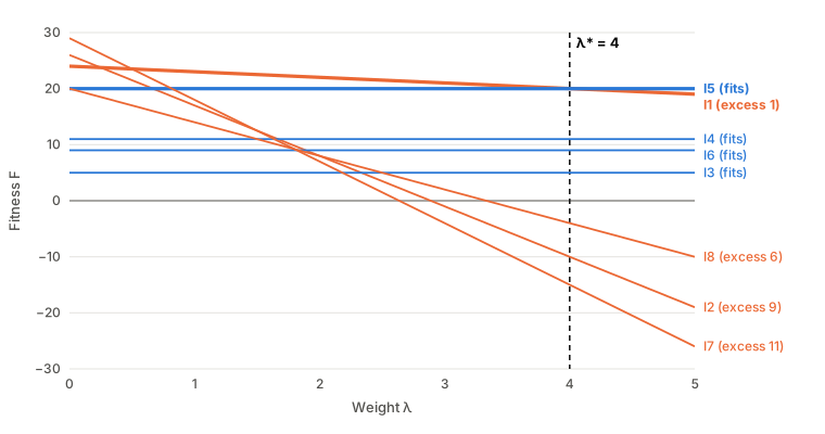
figuras/04-inicializar-evaluar.py in the book repository.
Show the figure data
| Individual | Fits? | Fitness with λ | λ = 0 | λ = 1 | λ = 4 | λ = 5 |
|---|---|---|---|---|---|---|
| I1 | No | 24 - \lambda | 24 | 23 | 20 | 19 |
| I2 | No | 26 - 9\lambda | 26 | 17 | −10 | −19 |
| I3 | Yes | 5 | 5 | 5 | 5 | 5 |
| I4 | Yes | 11 | 11 | 11 | 11 | 11 |
| I5 | Yes | 20 | 20 | 20 | 20 | 20 |
| I6 | Yes | 9 | 9 | 9 | 9 | 9 |
| I7 | No | 29 - 11\lambda | 29 | 18 | −15 | −26 |
| I8 | No | 20 - 6\lambda | 20 | 14 | −4 | −10 |
λ* depends on the population, which changes each generation. Hence dynamic penalties, whose weight increases with generations (Joines & Houck, 1994), and adaptive penalties, which adjust it to search progress. For example, raise it if the best individual has been infeasible throughout recent generations and lower it if the best has always been feasible (Hadj-Alouane & Bean, 1997; Michalewicz & Schoenauer, 1996, Section 3.2.4; Talbi, 2009, pp. 50–51). Other methods avoid choosing λ. In Deb’s tournament (2000), a feasible individual always beats an infeasible one. Between feasible individuals, the better objective wins; between infeasible individuals, the smaller violation wins. Also, with λ = 5, I2, I7, and I8 have negative fitness: roulette-wheel selection would require adding a constant, as in section 4.6.
Using the same population and the quadratic penalty, F = \text{value} - (\lambda\, e)^2: (a) what is the critical weight? (b) With λ = 3, what is I1’s fitness, and who is best? (c) With the linear penalty and λ = 2, who is best?
Show the solution
I1 falls below I5 if 24 - (\lambda \times 1)^2 < 20, that is, if \lambda^2 > 4: \lambda^* = \sqrt{4}/1 = 2. For the other infeasible individuals, \sqrt{z_i - B}/e_i is \sqrt{6}/9 \approx 0.27, \sqrt{9}/11 \approx 0.27, and 0. The critical weight is 2: I1 ties with I5 there, and λ > 2 is required to put it strictly below.
F = 24 - 3^2 = 15. The other infeasible individuals fall much lower (for example, I2: 26 - 27^2 = -703). I5 is best, with 20.
With the linear penalty, λ = 2 is below λ* = 4: I1 has F = 24 - 2 = 22 > 20 and remains best.
Explore in initialization-and-evaluation-ga
- Adjust Weight λ, move to the end (or click Play), and watch Penalty in this population. At what value does the best individual change?
- Set Penalty to quadratic and compare the lines at Penalty weight λ.
- Switch to Assignment · binary matrix, a minimization problem. What happens to λ* if the population contains no feasible individual?
4.8 The Cost of Evaluation BasicB
So far, we have evaluated one population. What does evaluation cost over an entire run?
In many problems, evaluation consumes most of a metaheuristic’s runtime (Jin, 2005; Talbi, 2009, p. 47). In aerodynamic design, for example, evaluating a structure requires a fluid dynamics simulation that may take more than a day, even on a parallel computer (Talbi, 2009, p. 47). Selection, crossover, and mutation cost very little by comparison.
A generational genetic algorithm evaluates N individuals each generation. With G generations plus the initial population, this gives N\,(G + 1) evaluations. This number is the algorithm’s budget. A fair comparison between algorithms counts evaluations, rather than generations or seconds on a particular computer (Eiben & Smith, 2015, pp. 152–153). A maximum number of evaluations is therefore a common stopping criterion (Section 8.6).
Many evaluations are repeated. Selection copies good individuals, and mutation leaves many offspring identical to their parent. With mutation probability 1/L per gene, the probability of no change is (1 - 1/L)^L, approaching 1/e \approx 0.37 as L grows. A cache, a table storing chromosomes and their fitness values, avoids evaluating a previously seen individual again: look it up before evaluating (Kratica, 1999).
Data. The population from example 4.3 (N = 8) evolves for G = 6 generations with a minimal algorithm: binary tournament and mutation of each gene with probability 1/L (1/6 with 6 items), without crossover. Evaluations are counted with and without caching.
Predict. What is the budget? How many evaluations do you think caching saves? With that same budget, how many generations could caching allow? Would it save as much with a 12-item knapsack?
Show the result
The budget is 8 \times (6 + 1) = 56 evaluations. With caching, the 6-item knapsack needs only 25, saving 31 (55%). The same budget of 56 would reach generation 55. In a space of only 64 chromosomes, without crossover, the population soon fills with previously evaluated chromosomes; after generation 24, hardly any new ones appear. This is an extreme case. With 12 items (2^{12} = 4\,096 chromosomes), caching requires 40 evaluations, saves 16 (29%), and reaches generation 9.Show the tool here (6 items)
Caching has conditions. It requires deterministic fitness: evaluating the same individual twice must give the same result. We examine this in section 4.13. It uses memory, one entry per distinct individual. The cache key also matters: in the traveling salesman problem, the 2n chromosomes representing the same tour have equal length, so caching by tour would save more than caching by chromosome. Other ways to save evaluations include parallel evaluation and replacing some evaluations with an approximate model, discussed in Further Reading.
(a) An algorithm with N = 50 individuals runs for 100 generations. How many evaluations does it perform? If each is a one-minute simulation, how long does it take? (b) With mutation probability 1/L per gene, what is the probability that an offspring has no changes if L = 6? What if L = 100?
Show the solution
50 \times 101 = 5\,050 evaluations, about 5 050 minutes: more than 84 hours, or three and a half days without stopping.
With L = 6, (5/6)^6 \approx 0.33. With L = 100, (0.99)^{100} \approx 0.37. In both cases, about a third of offspring that do not undergo crossover are exact copies of their parent.
Explore in initialization-and-evaluation-ga
- Advance generation by generation and record how many individuals were already cached. Does the number increase or decrease?
- Change Generations (G) and Problem and encoding. In which problem does caching save least?
Summary
- Generate the initial population uniformly at random: bits, integers, and real numbers gene by gene; permutations by Fisher–Yates shuffling. It should be diverse; it need not be good.
- Measure diversity with normalized distances between individuals. A uniform population over chromosomes is not uniform over feasible solutions: it may contain many infeasible individuals.
- Seeding with a heuristic may help, but it can also concentrate search around a few solutions. Protect diversity and check the effect in the full algorithm.
- Evaluation means decoding, calculating the objective, measuring violation, and combining these into fitness. A penalty weight λ should be neither too small, allowing infeasible individuals to win, nor too large.
- For roulette-wheel selection, transform cost into fitness (C - f, 1/(1 + f), or ranks). These preserve ordering but divide the wheel differently. Measure effort in evaluations, N\,(G + 1). A cache avoids repeated evaluations when fitness is deterministic.
To continue the basic path, go to “Selecting Parents”.
4.9 Covering the Box: Quasi-Random Sequences and Latin Hypercube Sampling AdvancedA
A uniform population spreads individuals evenly on average. Does it do so in each particular population, when there are only eight individuals?
No. With few individuals, chance leaves large gaps in some areas and clusters in others. Divide each axis of the box into N equal strips. A random point falls outside a given strip with probability 1 - 1/N, and N points leave it empty with probability (1 - 1/N)^N. With N = 8, this is 0.34: on average, a third of each axis’s strips remain empty. As N grows, the probability approaches 1/e \approx 0.37.
Two families of methods spread the population more evenly (Kazimipour et al., 2014; Talbi, 2009, pp. 194–196):
- Quasi-random, or low-discrepancy, sequences (Niederreiter, 1992) aim for points to spread out, rather than merely drawing independent numbers: new points fill gaps left by earlier ones. In general, they provide more diversity than pseudorandom numbers (Talbi, 2009, p. 195). Halton’s sequence (1960) uses the radical inverse of i in a different prime base for each coordinate (2 and 3 in the plane): write i in that base and reverse its digits after the decimal point. In base 2, i = 1, 2, 3, 4 gives 0.5, 0.25, 0.75, and 0.125: first the midpoint, then the missing quarters, then the eighths. Sobol’s sequence (1967) uses base 2 for all coordinates, combined differently. Both are deterministic: they always produce the same population. Maaranen et al. (2004) used them to generate a genetic algorithm’s initial population.
- Latin hypercube sampling (McKay et al., 1979) is random. Divide each axis into N equal strata; two random permutations decide which stratum each individual occupies on each axis, then sample its position within that stratum. Each stratum of each axis receives exactly one individual, like N nonattacking rooks on an N \times N chessboard. Talbi presents it as parallel diversification, because all solutions are generated together and independently, without evaluating the objective function (Talbi, 2009, pp. 195–196).
Data. The Himmelblau function in the box [-5, 5]^2 and N = 8 individuals from the Halton sequence, with x_j = -5 + 10\,u_j, rounded to two decimal places. The tool compares them with the uniform population of 8 individuals from the same seed.
Predict. Which points correspond to i = 1, 2, 3 and 4? How many of each axis’s 8 strips does Halton occupy? What about the uniform population?
Open: the second point Open: occupied strips
Show the result
| i | Base 2 | u_1 | Base 3 | u_2 | Point |
|---|---|---|---|---|---|
| 1 | 1 | 0.1₂ = 0.5 | 1 | 0.1₃ = 1/3 | (0.00, −1.67) |
| 2 | 10 | 0.01₂ = 0.25 | 2 | 0.2₃ = 2/3 | (−2.50, 1.67) |
| 3 | 11 | 0.11₂ = 0.75 | 10 | 0.01₃ = 1/9 | (2.50, −3.89) |
| 4 | 100 | 0.001₂ = 0.125 | 11 | 0.11₃ = 4/9 | (−3.75, −0.56) |
Show the tool here (occupied strips)
Figure 4.2 compares the three populations of eight individuals.
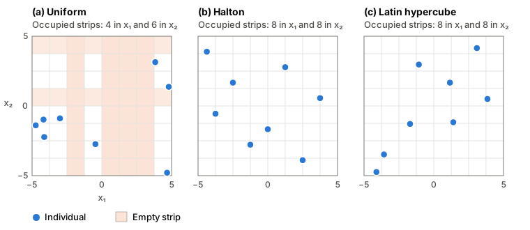
figuras/04-inicializar-evaluar.py in the book repository, using the points produced by initialization-and-evaluation-ga with population seed 1.
Show the figure data
| Individual | Uniform | Halton | Latin hypercube |
|---|---|---|---|
| 1 | (−4.13, −2.23) | (0.00, −1.67) | (3.85, 0.50) |
| 2 | (−0.46, −2.74) | (−2.50, 1.67) | (1.40, −1.17) |
| 3 | (4.80, 1.37) | (2.50, −3.89) | (1.16, 1.67) |
| 4 | (4.68, −4.79) | (−3.75, −0.56) | (−1.07, 2.97) |
| 5 | (−3.00, −0.89) | (1.25, 2.78) | (3.09, 4.15) |
| 6 | (−4.74, −1.39) | (−1.25, −2.78) | (−1.70, −1.29) |
| 7 | (3.83, 3.14) | (3.75, 0.56) | (−3.57, −3.48) |
| 8 | (−4.18, −0.98) | (−4.37, 3.89) | (−4.11, −4.74) |
In a genetic algorithm, the advantage is modest and is most noticeable with small populations and continuous problems with few variables. Experimental comparisons appear in Maaranen et al. (2004) and in the review by Kazimipour et al. (2014). Latin hypercube sampling does not guarantee good coverage of the plane: all eight points could lie on a diagonal while still occupying every strip. Halton and Sobol, as defined here, always give the same population, so independent runs (Section 9.3) require randomizing them.
Calculate u_1 and u_2 in the Halton sequence for i = 5, 6, and 7, and their corresponding points in [-5, 5]^2.
Show the solution
| i | Base 2 | u_1 | Base 3 | u_2 | Point |
|---|---|---|---|---|---|
| 5 | 101 | 0.101₂ = 5/8 = 0.625 | 12 | 0.21₃ = 2/3 + 1/9 = 7/9 | (1.25, 2.78) |
| 6 | 110 | 0.011₂ = 3/8 = 0.375 | 20 | 0.02₃ = 2/9 | (−1.25, −2.78) |
| 7 | 111 | 0.111₂ = 7/8 = 0.875 | 21 | 0.12₃ = 1/3 + 2/9 = 5/9 | (3.75, 0.56) |
Explore in initialization-and-evaluation-ga
- Change Method to Sobol sequence and Latin hypercube, and compare occupied strips and the largest gap.
- With Halton, click Draw the population. Does anything change? What about Latin hypercube?
- Click Compare strategies: the tool generates 1 000 populations per strategy. Which occupies more strips on average? Which gives the best initial individual?
4.10 Sequential Diversification AdvancedA
In the population from example 4.1, I4 = (2, 1, 1, 3, 1) and I6 = (3, 1, 1, 3, 1) differ at only one gene. Can we prevent such similar individuals from entering the population?
In sequential diversification, solutions are generated one after another to optimize diversity (Talbi, 2009, p. 195). The simplest method is simple sequential inhibition (SSI). It comes from spatial statistics, where it generates point patterns whose points cannot be too close together (Diggle, 1983). In a genetic algorithm, it works as follows: draw a candidate uniformly at random; accept it only if its distance from every individual already accepted is at least δ. Otherwise, discard it and draw another. Repeat until the population is complete (Talbi, 2009, p. 195).
By construction, the final population has a minimum distance of at least δ between individuals. The drawback is its relatively high cost and the unknown number of candidates needed (Talbi, 2009, p. 195). If δ is too large for the space and population size, N sufficiently separated individuals may not fit, and the process may never finish. After 50N candidates, the tool accepts subsequent candidates without checking distance. In practice, choose δ somewhat below a uniform population’s mean distance. Unlike quasi-random sequences and Latin hypercube sampling, SSI needs only a distance measure, so it works with any representation.
Data. The assignment problem from section 4.1, N = 6, and δ = 0.6: two individuals must differ at least at 3 of their 5 genes. Candidates appear in the same order as the population from example 4.1: (1, 1, 2, 1, 3), (2, 3, 1, 1, 2), (1, 2, 3, 3, 1), (2, 1, 1, 3, 1), (1, 2, 2, 1, 2), (3, 1, 1, 3, 1)…
Predict. Which of these six candidates enter the population? How many candidates do you think will be needed in total?
Open: the fifth candidate Open: the cost
Show the result
The first four enter: their distances to the nearest previously accepted individual are 0.80, 0.80, and 0.60. The fifth, (1, 2, 2, 1, 2), is 0.40 from I1 (they differ at tasks 2 and 5) and is rejected. The sixth, (3, 1, 1, 3, 1), is 0.20 from the fourth and is also rejected. It takes 11 candidates to obtain 6 individuals: 5 are rejected. The population’s minimum distance increases from 0.20 under uniform initialization to 0.60, and its mean from 0.71 to 0.76.Show the tool here (the cost)
Sequential inhibition neither considers quality nor spreads the population evenly over the entire space: it only prevents individuals from being too close.
(a) Calculate the distance from the fifth candidate in example 4.10, (1, 2, 2, 1, 2), to each of the four accepted individuals. (b) Would it have been accepted with δ = 0.4? (c) For which δ values would the population be exactly the uniform population from example 4.1?
Show the solution
Compared with I1 = (1, 1, 2, 1, 3), tasks 2 and 5 change: 2/5 = 0.4. Compared with I2 = (2, 3, 1, 1, 2), tasks 1, 2, and 3 change: 0.6. Compared with I3 = (1, 2, 3, 3, 1), tasks 3, 4, and 5 change: 0.6. Compared with I4 = (2, 1, 1, 3, 1), all five change: 1. The nearest distance is 0.4.
Yes: 0.4 ≥ 0.4.
The uniform population consists of the first six candidates, with a minimum distance of 0.20 (between the fourth and sixth). For any δ of 0.20 or less, all six enter and the population is uniform, because the rule is “at least δ.” With δ = 0, sequential inhibition is uniform initialization.
4.11 Feasible Initialization AdvancedA
If almost every random chromosome is infeasible under some encodings, can we generate a population that satisfies the constraints directly?
Yes, by changing what we sample. For the knapsack, shuffle the items using Fisher–Yates (Section 4.2), then process them in that order, including each if it fits in the remaining capacity. The result is always feasible and full: no further item fits. Chu & Beasley (1998) used this type of initialization in their genetic algorithm for the multidimensional knapsack. For the assignment binary matrix, simply draw each task’s machine, j = 1 + \lfloor u\,m \rfloor, and place a single 1 in that column of its row. This is uniform initialization of the integer vector, written as a matrix. Initial feasibility depends on both representation and method.
Feasible initialization has a price. Filling knapsacks biases the population: solutions with few items never appear, even though they are feasible and may carry valuable genes, and individuals are more similar. With complex constraints, finding even one feasible solution may be as hard as solving the problem. It is then more practical to handle constraints during evaluation with penalties (Section 4.7), or with repairs and decoders (Section 3.10). Rejecting infeasible solutions is reasonable only when they occupy a very small part of the search space (Talbi, 2009, p. 49).
Data. The knapsack from section 4.3 (W = 13). For the first individual, the shuffled item order is 2, 4, 3, 5, 1, 6.
Predict. Which items enter? What are the knapsack’s weight and value? Is it full?
Open: the first individual Open: population quality
Show the result
| Item | Weight | Cumulative weight if included | Fits? |
|---|---|---|---|
| 2 | 3 | 3 | Yes |
| 4 | 8 | 11 | Yes |
| 3 | 5 | 16 | No |
| 5 | 4 | 15 | No |
| 1 | 4 | 15 | No |
| 6 | 2 | 13 | Yes |
Show the tool here (the first individual)
The tool’s “Compare strategies” view repeats each strategy over 1 000 populations of this knapsack, with N = 8. On average, feasible initialization gives 100% feasible individuals (versus 53% under uniform initialization) and a best initial value of 20.4 (versus 17.3), but only 68% distinct individuals (versus 95%). Seeding half the population with the greedy solution gives 61% distinct individuals and a minimum distance of 0. Sequential inhibition with δ = 0.30 is the only method that increases diversity, at the cost of generating 1.6 times as many candidates.
For the same knapsack: (a) which individual results from shuffled order 3, 5, 1, 2, 6, 4? (b) Can this initialization produce 1 0 0 0 0 0? (c) What about the greedy solution, 0 0 1 0 1 1?
Show the solution
Include item 3 (weight 5), item 5 (9), and item 1 (13); items 2, 6, and 4 no longer fit. The result is 1 0 1 0 1 0, the optimum.
No. With only item 1 (weight 4), other items still fit, and the procedure would have included them. It produces only full knapsacks.
Yes. With items 3, 5, and 6, the knapsack weighs 11 and has 2 units left. No remaining item fits (the lightest weighs 3), so it is full. Order 6, 3, 5, 1, 2, 4 produces it, for example.
Explore in initialization-and-evaluation-ga
- Switch to Assignment · binary matrix and compare feasibility with uniform initialization.
- Open Compare strategies with this knapsack. Find the strategy with the most distinct individuals and the one with the best initial individual. Are they the same?
4.12 Fitness Landscapes AdvancedA
In some problems, a few changes always lead to the optimum; in others, any search gets stuck. What makes the difference?
Imagine each chromosome at a height equal to its fitness: valleys, peaks, plateaus, and cliffs appear. This is the fitness landscape. The idea comes from population genetics: Wright (1932, pp. 357–358) proposed it to study evolution (Talbi, 2009, p. 104). Three things define it: representation, the neighborhood specifying which chromosomes are reachable through a small change, and the objective function (Stadler, 2002; Talbi, 2009, p. 104). The landscape is therefore not a property of the problem alone: change the representation or neighborhood, and the same problem has a different landscape.
A local optimum is a chromosome with no better neighbor. A local search that always moves to the best neighbor ends at the local optimum of its starting basin. With many local optima—a rugged landscape—different starting points lead to different optima and rarely to the global one (Kauffman & Levin, 1987). A genetic algorithm moves an entire population through the landscape, and crossover can jump between basins. Yet landscape structure still affects difficulty; this is why a diverse initial population starts in many basins at once.
To summarize landscape structure without plotting it, Jones & Forrest (1995) proposed fitness–distance correlation (FDC): the correlation between many chromosomes’ fitness and their distance to the nearest global optimum (Talbi, 2009, pp. 114–115). For minimization, a strong positive correlation indicates a relatively easy problem (fitness improves toward the optimum); a strong negative correlation indicates deception; a value near zero means fitness provides little guidance. Its major limitation is the need to know the optimum, which is unrealistic for many problems (Talbi, 2009, p. 115). Malan & Engelbrecht (2013) review other landscape measures, such as fitness autocorrelation along a random walk, that do not require it.
Data. The assignment problem from section 4.1 and its one-gene neighborhood: two assignments are neighbors if moving one task to another machine turns one into the other. Local search starts at I1 = (1, 1, 2, 1, 3), with makespan 21, and moves to the best neighbor at each step. Ties are broken by task order, then machine order within each task.
Predict. How many neighbors does each assignment have? How many improve on I1? Will local search reach the optimum, 5?
Open: I1’s neighbors Open: local search
Show the result
Each task can move to two other machines: 5 \times 2 = 10 neighbors. Of I1’s neighbors, 6 are better; the best moves task 2 to machine 2, reducing makespan to 12. Local search proceeds as follows:
| Step | Assignment | Move | Makespan |
|---|---|---|---|
| 0 | (1, 1, 2, 1, 3) | 21 | |
| 1 | (1, 2, 2, 1, 3) | task 2 to machine 2 | 12 |
| 2 | (1, 2, 2, 3, 3) | task 4 to machine 3 | 11 |
| 3 | (1, 2, 1, 3, 3) | task 3 to machine 1 | 7 |
Show the tool here (local search)
Check that assignment (1, 2, 1, 3, 3), where the search in example 4.12 ends, is a local optimum. (a) Calculate its loads. (b) Which task would need to move to reduce makespan below 7? Is moving one enough? (c) How many neighbors also have makespan 7?
Show the solution
Machine 1 handles tasks 1 and 3: 5 + 2 = 7. Machine 2 handles task 2: 2. Machine 3 handles tasks 4 and 5: 1 + 5 = 6. Makespan is 7.
To get below 7, we must reduce machine 1’s load by moving task 1 or 3. Moving task 1 to machine 2 gives 2 + 5 = 7; moving it to machine 3 gives 6 + 8 = 14. Moving task 3 to machine 2 gives 2 + 9 = 11; moving it to machine 3 gives 6 + 1 = 7. No single-task move gets below 7, so it is a local optimum. Reaching the optimum, (1, 2, 3, 3, 2), requires moving two tasks: task 3 to machine 3 and task 5 to machine 2.
Four neighbors also have makespan 7: task 1 to machine 2, task 3 to machine 3, task 4 to machine 2, and task 5 to machine 2. This is a plateau: local search that accepts only improving neighbors stops there.
Explore in initialization-and-evaluation-ga
- With Himmelblau, see how many local searches reach a minimum. Change Function to Rastrigin and repeat. Which landscape is rugged?
- Switch to 2D function · bit string. With the same function, how many local optima appear now? Recall the jumps in section 3.8.
4.13 Noisy Fitness AdvancedA
What if evaluating the same individual twice produces different numbers?
In many real problems, data contain noise. Fitness may come from a stochastic simulator or a sensor, or data may be uncertain: variable processing times in scheduling or random demands along a route, for example (Talbi, 2009, p. 15). We can write \tilde F(x) = f(x) + \varepsilon, where ε is noise, often assumed normal with mean 0 and standard deviation σ. In practice, fitness is approximated by averaging several evaluations (Talbi, 2009, p. 15).
With noise, selection compares values that differ from true fitness. If the true difference Δ between two individuals is small relative to σ, their apparent ordering is almost a coin toss. The mean of R evaluations has the same expected value and standard deviation \sigma/\sqrt{R}. The difference between two individuals’ means therefore has standard deviation \sigma\sqrt{2/R}, and the probability of ordering them incorrectly is \Phi\!\left(-\frac{\Delta\sqrt{R}}{\sigma\sqrt{2}}\right), where Φ is the standard normal cumulative distribution function. Reevaluation has a cost: N individuals evaluated R times require N \times R evaluations per generation, and halving the error requires four times as many.
Data. A uniform population of 8 points on the Himmelblau function, to be minimized. The two best are I1, with true fitness 52.555, and I7, with 91.112: a difference Δ ≈ 38.56. Each evaluation adds normal noise with σ = 30. Compare one evaluation per individual with the mean of R = 5.
Predict. What is the probability of ordering I1 and I7 incorrectly with one evaluation? What about the mean of 5? How many evaluations does each option require?
Show the result
With one evaluation, \Delta/(\sigma\sqrt 2) = 38.56/42.43 \approx 0.91 and \Phi(-0.91) \approx 18.2%. With the mean of 5, multiply the argument by \sqrt 5: \Phi(-2.03) \approx 2.1%. The price is 40 evaluations rather than 8. To get below 5%, 4 evaluations per individual suffice. In this population, incorrectly ordered pairs fall from 5 to 2 out of 28.Show the tool here (the cost)
Noise changes other decisions too. The cache from section 4.8 no longer works as described: it would preserve a lucky evaluation forever. Elitism (Section 8.3) can retain an individual that merely appeared good. The final solution should be evaluated several times before accepting it. Cheaper alternatives to reevaluating everyone include increasing population size, which implicitly averages noise, or reevaluating only individuals involved in close comparisons. Jin & Branke (2005) review these techniques.
With the data from example 4.13 (Δ = 38.56, σ = 30), how many evaluations per individual make the probability of ordering I1 and I7 incorrectly less than 5%? Use \Phi(-1.645) = 0.05.
Show the solution
We need \Delta\sqrt{R}/(\sigma\sqrt 2) \ge 1.645, or 0.909\,\sqrt R \ge 1.645, \sqrt R \ge 1.81, and R \ge 3.27. Since R is an integer, R = 4. With N = 8, that means 32 evaluations per generation instead of 8.Explore in initialization-and-evaluation-ga
- Change Noise (σ) and Evaluations per individual (R), and watch how many pairs are ordered incorrectly.
- Switch to TSP · permutation. What σ makes the apparent best individual differ from the true best?
4.14 Further Reading Further reading+
Approximate fitness. When an evaluation takes hours, some evaluations can be replaced with a meta-model: a cheap function approximating the objective from a sample of previously evaluated solutions. This is also called a surrogate model or approximate fitness. Neural networks, response surfaces, kriging, and Gaussian processes are common meta-models (Jin, 2005, 2011; Talbi, 2009, pp. 47–48). The tradeoff is familiar: exact, expensive evaluation versus cheap evaluation with error; the two can be alternated (Talbi, 2009, p. 48). A typical use is preselection: the meta-model identifies promising candidates from a larger set, and only those are evaluated exactly. In the tool’s “Approximate fitness” view, an inverse-distance-weighting meta-model built from the initial population’s 8 individuals ranks 8 new candidates rather poorly (rank correlation 0.26). Yet evaluating only its estimated best 4 saves 4 evaluations and includes the true best candidate.
Multiple objectives. Many real problems have conflicting objectives: a more valuable knapsack weighs more. There is then no single solution better than all others, but a set of tradeoffs. One solution dominates another if it is no worse in any objective and better in at least one. Solutions dominated by no other solution in the search space are Pareto optima (Deb, 2001; Talbi, 2009, p. 311). Within a population, “nondominated” means only that no other member of that population dominates it. There are two ways to evaluate. A weighted sum normalizes and combines objectives using weights, turning the problem into a single-objective problem. Its drawback is that it finds only supported solutions: no choice of weights selects solutions in a nonconvex part of the front (Talbi, 2009, pp. 324–325). Alternatively, fitness can be assigned by dominance. Nondominated individuals form the first front; remove them, and the remaining nondominated individuals form the second, and so on. In “Several objectives”, using the population from example 4.3 without the knapsack’s capacity constraint (maximize value and minimize weight), the first front has 6 individuals, and no choice of weights selects 2 of them.
Without the capacity constraint, each individual in example 4.3 has two objectives: value, to be maximized, and weight, to be minimized. Which individuals are dominated, and by whom?
Show the solution
The pairs (value; weight) are I1 (24, 14), I2 (26, 22), I3 (5, 4), I4 (11, 7), I5 (20, 11), I6 (9, 12), I7 (29, 24), and I8 (20, 19). I6 is dominated by I4 (higher value and lower weight) and by I5. I8 is dominated by I5 (equal value and lower weight) and by I1. The other six form the first front.For the history of multiobjective genetic algorithms, from early methods to more recent ones, and further reading, see “Multiple Objectives” in section 11.6.
A population diverse by construction. Generating the initial population can itself be an optimization problem: choose N solutions that maximize a diversity measure, such as the smallest distance between any pair. This can be as difficult as the original problem, so approximate methods are used. For example, generate part of the population at random, then add solutions one at a time, choosing those farthest from the individuals already present (Talbi, 2009, pp. 194, 197–198).
Relative fitness. Some problems have no absolute value to measure. In a game, for example, strategy A may beat B, B beat C, and C beat A. Fitness then comes from comparing individuals, through ranks or competitions. This is enough for population algorithms, because selection needs only to know who is better (Talbi, 2009, p. 47).
More to read. Kazimipour et al. (2014) review population initialization techniques in evolutionary algorithms; Coello Coello (2002) reviews constraint-handling methods.