9 Parameters and Randomness
Tools: EvoTraveller and SelectionMechanisms, available through the portal. Both have English-only interfaces.
After completing the basic path through this chapter, you will be able to:
- explain why two runs of the same genetic algorithm give different results and what role the seed plays;
- calculate the mean and standard deviation of several runs and interpret them;
- explain why a difference between single runs may be due to chance and why the means of several replicates must be compared;
- explain why there are no values of Pc and pm that are good for every problem and how to tune them with cases similar to the real one;
- relate selection pressure to loss of diversity and to mutation.
9.1 An Algorithm That Depends on Chance BasicB
If we run the same genetic algorithm twice, do we get the same solution?
A genetic algorithm uses random numbers in almost every step: to create the initial population, to choose parents (chapter 5), to decide whether a pair is crossed over and where (chapter 6), and to decide which individuals mutate and how (chapter 7). It is a stochastic algorithm: with the same data and the same parameters, each run can end up in a different place.
On a computer, “random” numbers are produced by a generator that starts from an initial value, the seed. With the same seed, the generator always gives the same sequence, and the run is repeated identically; with another seed, it is another run. Fixing the seed lets us reproduce a result, but it does not make the result more reliable: it is one run among many possible ones.
EvoTraveller solves the traveling salesman problem with a genetic algorithm (Santos et al., 2025). There is an origin at position (0, 0) and several places scattered over a grid; the algorithm looks for the shortest route that passes through all of them and returns to the origin. Each individual is a permutation of the places, and its fitness is the inverse of the route length, so higher fitness means a shorter route. It uses tournament selection, permutation crossover and mutation, and generational replacement with an elite, as in the previous chapters. With 10 places, the origin and 9 others, there are 9! = 362 880 possible routes. A separate program checks them all and tells us which is best, with length 31.50. With that figure, we can measure how far from the optimum the algorithm ends up.
EvoTraveller Reference Settings
These are the starting values for the examples. Before each activity, check the eight controls and change only those the activity mentions. An earlier activity may have left them with other values.
| Control | Reference value |
|---|---|
| Number of places | 10 |
| Seed | 1111 |
| Population size | 100 |
| Generations | 50 |
| Tournament size | 4 |
| Mutation rate | 0.05 |
| Elitism | 0.05 |
| Crossover | 0.6 |
If Zzzz appears when you open EvoTraveller, the application is asleep: click Yes, get this app back up! and wait for the controls to appear. Then set the values and click Run. For a class, it is a good idea to open it before starting.
Data. In EvoTraveller, keep the reference values: Number of places 10, Seed 1111, Population size 100, Generations 50, Tournament size 4, Mutation rate 0.05, Elitism 0.05, and Crossover 0.6. Click Run.
Predict. Does the algorithm find the best possible route, of length 31.50? If you click Run again without changing anything, which route will you get?
Open and configure: EvoTraveller
Show the result
The Fitness curve rises from 0.0230 in generation 0 to 0.0293 at the end, and it stops improving around generation 3. The inverses of those values are the route lengths: from 43.45 to 34.11. The optimum is 31.50, so the route found is 8.3% longer.
If you click Run again, you get exactly the same route: the seed is the same, and the generator repeats the same sequence of numbers.Change only the Seed to 1112 and click Run. What has changed: only the algorithm’s random numbers, or the problem as well? What does this imply for comparing two runs with different seeds?
Show the solution
In EvoTraveller, the seed fixes both the algorithm’s random numbers and the positions of the places, so with another seed the map changes too: it is another problem, and its best route may be longer or shorter. Comparing two runs with different seeds mixes the effect of the algorithm’s randomness with the difficulty of each map. To compare two configurations, you must use the same seed, and therefore the same map, and change only the parameter.9.2 Crossover and Mutation Probabilities BasicB
How much should we cross over, and how much should we mutate?
Chapters 6 and 7 introduced two parameters that control how much the population changes in each generation. The crossover probability Pc is the probability that a pair of parents is crossed over; if it is not, its offspring are copies of the parents. The mutation probability pm is the probability that a gene or, in a permutation, an individual mutates (Eiben & Smith, 2015). In EvoTraveller, Mutation rate is pm: each individual except the elite mutates with that probability, by swapping two places. Crossover plays the role of Pc: it is the fraction of the population formed by crossover; the rest are copies of the parents, which can also mutate. The elite (Elitism) is another fraction of the population: the best individuals, which pass into the next generation without being crossed over or mutated (Santos et al., 2025, p. 9), as we saw in section 8.3. Pc and pm are only two of the algorithm’s parameters. The others are the population size, the tournament size, the elite fraction, and the number of generations.
Remember that pm does not mean the same thing in every representation. With bits, pm is the probability that each gene mutates. The usual values are small, from 0.001 to 0.01, or \mathit{pm} = 1/L, where L is the number of genes, so that on average only one gene mutates in each individual (Talbi, 2009, p. 208). We saw this in section 7.7. In EvoTraveller, by contrast, pm is the probability that the individual receives a swap, which changes two positions. On average, each child changes 2 \times \mathit{pm} positions: with pm = 0.05, a tenth of a position; with pm = 0.5, one position, as the 1/L rule asks. To compare values of pm across representations, they must be translated into how many genes change, on average, in each child.
Data. The same problem as in example 9.1, with all the reference values except Mutation rate, which takes three values: 0; 0.05; and 0.2. Click Run with each one.
Predict. With which value does the route end up shortest? And longest?
Open and configure: EvoTraveller
Show the result
| Mutation rate | Final fitness | Final length | Above the optimum (31.50) |
|---|---|---|---|
| 0 | 0.0261 | 38.34 | +21.7% |
| 0.05 | 0.0293 | 34.11 | +8.3% |
| 0.2 | 0.0317 | 31.50 | 0% |
But be careful: this is one run with each value. That 0.2 won here does not tell us that it is better in general. We will see this in the next sections.
In example 9.2, without mutation, the best fitness stops improving around generation 5. Why does it not keep improving, if crossover keeps combining routes?
Show the solution
Selection only copies routes that already exist. When the population fills up with copies of a few routes, many recombinations stop producing improvements. EvoTraveller’s OX, “Order from the start”, can create another route even when it crosses two copies, because it is not pure (example 6.11); but a new route need not be better. Mutation provides another way of varying the routes. In section 10.4 we will see why the changes made by crossover are not enough in this run.9.3 One Run Is Not Enough BasicB
If the result depends on chance, how do we know what a genetic algorithm achieves in general?
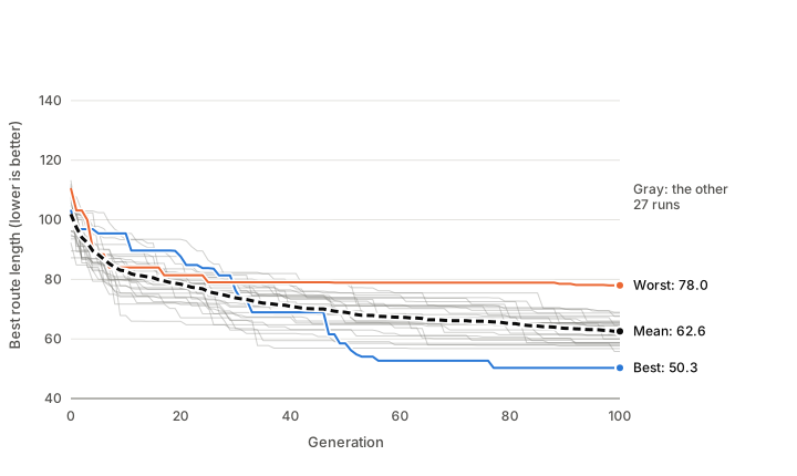
By repeating the run. Each repetition with a different seed is a replicate, and what interests us is how the results of many replicates are distributed. EvoTraveller does not allow repeated runs on the same map, because the seed also changes the map. That is why we have programmed an algorithm with the same design: permutations, a tournament of 3, OX crossover with Pc = 0.6, swap mutation with pm = 0.05 per individual, and generational replacement with one elite individual. In our program we use the classic OX from section 6.6; EvoTraveller uses “Order from the start”. They share the general components, but they do not reproduce the same implementation or the same draws. We applied it to a map with 20 destinations and the origin, where the route starts and ends: 21 cities in total. In EvoTraveller, Number of places also counts the origin, so this map would be 21 places, more than the 15 it allows. We used a population of 30 and 100 generations. One map, 30 different seeds (1 to 30).
figuras/09-experimentos.py in the book’s repository.
Show the figure data
Final length of the best route in the 30 runs, from lowest to highest: 50.3; 55.8; 56.8; 57.6; 57.9; 58.3; 58.7; 58.7; 58.8; 60.0; 60.0; 61.1; 61.2; 61.4; 61.5; 62.5; 63.4; 64.4; 64.6; 64.7; 65.1; 65.4; 65.4; 65.9; 66.0; 67.6; 67.7; 68.7; 69.0; 78.0.
The mean length of the best route goes from 101.9 in generation 0 to 68.9 in generation 50 and 62.6 in generation 100.All the runs improve, and quickly at first. But they do not end in the same place: the best finishes at 50.3 and the worst at 78.0. With a single run, the result could have been any one of those thirty.
Two numbers are used to summarize many replicates. The mean is the typical result, and the standard deviation measures how far the replicates stray from it:
\bar{x} = \frac{1}{n}\sum_{i=1}^{n} x_i, \qquad s = \sqrt{\frac{1}{n-1}\sum_{i=1}^{n} (x_i - \bar{x})^2}
where x_i is the result of replicate i and n is the number of replicates. In our 30 replicates, the mean final length is 62.6 and the standard deviation is 5.2. A small standard deviation indicates that the algorithm is robust: it gives similar results even when the randomness changes (Talbi, 2009, p. 63). If the spread is large, a particular run can turn out much worse than the mean, and whoever relies on it has no way of knowing.
Data. In EvoTraveller, with Number of places 15 and the other reference values, do one run with each seed, from 1111 to 1115, and with each Mutation rate: 0; 0.05; and 0.2. That makes 15 runs. The results table gives the final length; the fitness is its inverse.
Predict. Does 0.2 always beat the other two? And does 0.05 always beat 0?
Open and configure: EvoTraveller
Show the result
| Seed | Optimum | Mutation rate 0 | 0.05 | 0.2 |
|---|---|---|---|---|
| 1111 | 37.04 | 47.64 | 43.08 | 38.46 |
| 1112 | 39.81 | 46.98 | 46.52 | 45.72 |
| 1113 | 32.31 | 41.28 | 37.29 | 35.40 |
| 1114 | 34.49 | 43.84 | 38.99 | 37.03 |
| 1115 | 38.38 | 40.86 | 44.90 | 39.53 |
| Mean | 44.12 | 42.16 | 39.23 |
The first five replicates in figure 9.1, with seeds 1 to 5, end at 66.0; 56.8; 61.2; 58.7; and 57.9. Calculate their mean and standard deviation. Compare them with those of the 30 replicates (62.6 and 5.2). What would have happened if you had done only the run with seed 1?
Show the solution
The mean is (66.0 + 56.8 + 61.2 + 58.7 + 57.9)/5 = 60.12. The deviations from the mean are 5.88; −3.32; 1.08; −1.42; and −2.22, and their squares add up to 53.7. Divided by n - 1 = 4, this gives 13.4, and its square root is the standard deviation: 3.7.
With five replicates, the mean comes out somewhat lower than with 30 (60.1 versus 62.6) and the standard deviation somewhat smaller (3.7 versus 5.2): with few replicates, the estimates are unreliable. With seed 1 we would have obtained 66.0, which is above the mean of the 30 replicates: we would have overestimated the typical length of its routes (66.0 versus 62.6).9.4 Comparing Two Configurations BasicB
If one configuration gives a lower mean than another, is it better?
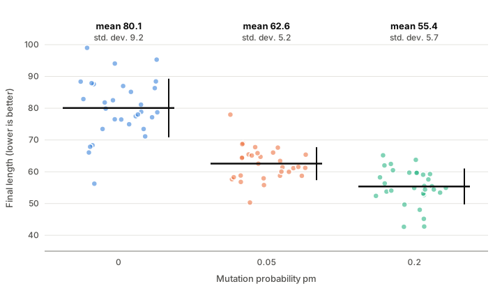
With the same map and the same 30 seeds, we repeated the experiment with three values of pm: 0; 0.05; and 0.2. All of them use the same map and the same 30 seeds, and therefore the same 30 initial populations.
figuras/09-experimentos.py in the book’s repository.
Show the figure data
| pm | Mean | Standard deviation | Minimum | Maximum |
|---|---|---|---|---|
| 0 | 80.1 | 9.2 | 56.2 | 99.0 |
| 0.05 | 62.6 | 5.2 | 50.3 | 78.0 |
| 0.2 | 55.4 | 5.7 | 42.7 | 65.2 |
The difference between 0 and 0.05 is large compared with the spread of the clouds. The difference between 0.05 and 0.2 is smaller and the clouds overlap, but it is still clear: the mean falls from 62.6 to 55.4. Because the three configurations use the same seeds, each seed forms a pair: two runs that start from the same initial population and differ only in pm. The natural comparison is made within each pair. With 0.05, the final route is shorter than with 0.2 for 3 of the 30 seeds, 10%; without mutation, it is shorter than with 0.05 for 1 of the 30.
We can also ask what would happen to someone who did a single run of each configuration, with different seeds for each one. To simulate this, we combine each run with 0.05 with each run with 0.2: 30 × 30 = 900 pairs. In 146 of them, 16%, the run with 0.05 ends with a shorter route. And the run without mutation beats the one with 0.05 in 5% of the 900 pairs (47).
If we had done a single run with each value, we would have wrongly concluded that 0.05 is better than 0.2 for 3 of the 30 seeds, and in one in six pairs with different seeds. With only 30 seeds, these two figures cannot really be told apart: here, sharing the seed fixes only the initial population and has little influence on the final result, as we will see in section 9.8. With 30 replicates, the mean of each configuration has a much smaller error, and the conclusion is reliable. Comparing means of several replicates, not single runs, is what makes a comparison credible.
There is one more condition: the comparison is valid only for what has been tested. Here, for this map, this population size, and these 100 generations. We do not yet know anything about other cases; we will come back to this in section 9.5.
A classmate compares pm = 0.05 and pm = 0.2 with a single run of each, with different seeds chosen at random. According to the 900 pairs in section 9.4, how often will they find that 0.05 is better? And if they use the same seed for both? And what would they find if they compared the means of 30 replicates?
Show the solution
With one run of each, 0.05 comes out better in 146 of 900 pairs, 16%: they would be wrong about once in every six comparisons. With the same seed, 0.05 comes out better for 3 of the 30 seeds. With so few pairs, this figure is compatible with 16%: in this algorithm, sharing the seed does not protect against being wrong. With the means of 30 replicates, the means are 62.6 and 55.4: the difference is 7.2, and the advantage of 0.2 holds. In section 9.8 we will see how to measure whether this difference is credible: it is about five times its standard error, so with 30 replicates it would almost never come out the other way around.9.5 Tuning with Similar Cases BasicB
Which values of Pc and pm should we use in a new problem?
There is no universal recipe. Suitable values depend above all on the problem, even on the particular instance, and on how much search time we want to spend; there is no set of values that is optimal for every case (Eiben & Smith, 2015, p. 124; Talbi, 2009, p. 54). The first systematic studies produced combinations that were widely used. De Jong, with a battery of test functions, found that the best was a population of 50 to 100 individuals, a Pc of 0.6 per pair, and a pm of 0.001 per bit (De Jong, 1975; according to Schaffer et al., 1989, p. 52). Grefenstette, with a genetic algorithm that tuned the parameters of another one, obtained a population of 30, Pc = 0.95, and pm = 0.01 (Grefenstette, 1986, p. 126). And Schaffer and his colleagues, after testing many combinations, obtained a population of 20 to 30, Pc between 0.75 and 0.95, and pm between 0.005 and 0.01 (Schaffer et al., 1989, p. 54). But those values were obtained with particular batteries of problems, and it is not known how well they hold outside them (Mitchell, 1996/1998, Section 5.6). A different criterion gives a different answer. Grefenstette himself found this. His values were the best for online performance, the mean of all the solutions evaluated during the search. For offline performance, which looks only at the best solution found up to each moment, the best configuration had 80 individuals and Pc = 0.45 (Grefenstette, 1986, pp. 125–126). Tuning with different measures can give values that differ by orders of magnitude, so a recommendation that does not say which measure it was obtained with should be taken with caution (Eiben & Smith, 2015, p. 126). Haupt and Haupt counted how many evaluations were needed to reach an acceptable solution on functions of two variables, and the best were small populations, of 8 to 20 individuals, with mutation rates between 0.03 and 0.37, depending on the function; the larger the population, the lower the best rate (Haupt & Haupt, 2004, pp. 131–132). The criterion matters: they stopped as soon as an acceptable solution was reached (Haupt & Haupt, 2004, p. 134), and what counts as a good value depends on what we are looking for (section 9.6). Moreover, their pm is per bit: with chromosomes of 24 bits, 0.11 means about 2.6 bits changed per child. And we have already seen that pm is defined differently in a permutation.
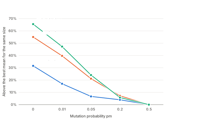
To see how much it depends on the problem, we repeated the experiment with three sizes: 10, 20, and 30 destinations, plus the origin, one map of each size, and 30 replicates per value of pm. Figure 9.3 does not show lengths, because they are not comparable across maps. For each size, it shows how much longer the mean for each value of pm is than that of the best of the five values tested.
figuras/09-experimentos.py in the book’s repository.
Show the figure data
Mean final length of 30 runs and, in parentheses, the percentage above the best mean on the same map:
| pm | 10 destinations | 20 destinations | 30 destinations |
|---|---|---|---|
| 0 | 41.8 (+32%) | 80.1 (+55%) | 123.9 (+66%) |
| 0.01 | 37.2 (+17%) | 72.1 (+40%) | 110.3 (+47%) |
| 0.05 | 33.9 (+7%) | 62.6 (+21%) | 92.9 (+24%) |
| 0.2 | 33.0 (+4%) | 55.4 (+7%) | 79.2 (+6%) |
| 0.5 | 31.8 (0%) | 51.6 (0%) | 74.9 (0%) |
On these three maps, a low value of pm, such as 0.05, fares worse on the larger ones. Because there is only one map per size, we cannot separate the effect of size from that of each map’s structure. With pm = 0.05, the mean is 7% above the best with 10 destinations, 21% with 20, and 24% with 30. Of the five values tested, the best is the same for all three sizes: 0.5. It is not a strange value: as we saw in section 9.2, it amounts to changing one position per child on average, which is what the 1/L rule asks for, and 0.05 amounts to mutating ten times less. EvoTraveller only goes up to 0.2. In section 9.9 we will see why this algorithm tolerates so much mutation. If we had tuned pm on the problem with 10 destinations, we would have believed that 0.05 is close to the best, but on the problem with 30 destinations it is not.
This leads to a practical rule: tune the parameters with cases similar to the real one, in size and in structure, not with a small, convenient case. And preferably with several cases rather than just one. This has a limit that we will see in the further reading: if we tune the parameters on some cases and evaluate the algorithm on the same ones, the result is too optimistic.
You have a real problem with 30 destinations, but to tune pm you use only the one with 10, because it is faster. With the data in figure 9.3, what difference do you see between pm = 0.05 and pm = 0.2 for each size? What conclusion would you draw from the small case about how much choosing pm well matters, and what would happen with the real one?
Show the solution
With 10 destinations, 0.05 and 0.2 are 7% and 4% above the best mean: only 3 points apart. With 30 destinations they are 24% and 6% above: 18 points. With the small case, the difference looks negligible, and we might think that we could just as well keep the usual value, 0.05. Applied to the problem with 30 destinations, we would lose much more: the route would be, on average, 24% longer than with the best value tested. In these examples, using only the small map would have underestimated how much pm matters on the large map.- With Number of places 10 and Mutation rate 0.05, do one run with each seed, from 1111 to 1115. Repeat with Mutation rate 0.2. For how many seeds does the route improve? With 10 places, going from 0.05 to 0.2 improves the route for only 2 of the 5 seeds (1111 and 1114); for the other 3, the final route is the same.
- Do the same with Number of places 15. For all five seeds, 0.2 gives a shorter route than 0.05. On these five maps with 15 places, the improvement appears more often than on those with 10; the pattern may change with other maps.
9.6 What Are You Looking For? BasicB
What is a good result: the best possible solution, or a good solution right away?
When tuning an algorithm, two measures are at stake: solution quality and search time. Which matters more depends on the problem. Talbi distinguishes three classes according to the weight of each (Talbi, 2009, pp. 33–34):
- Design or strategic problems. They are solved only once, the time available is long (hours, days, months), and a bad solution has lasting consequences, for example the design of a telecommunications network. Quality matters, and spending a lot on the search is justified.
- Control or operational problems. They must be solved frequently and in real time, with decisions in fractions of a second, for example routing messages in a network. Very fast heuristics are needed, and quality matters less.
- Planning or tactical problems. They lie between the two extremes, in the medium term. Quality and time must be balanced.
This translates into parameters. In a genetic algorithm, a larger population or more generations cost more evaluations and therefore more time, and repeating the run to obtain replicates multiplies the cost. The same algorithm with different values can be suitable for a design problem and useless for an operational one. That is why, before tuning parameters, we must ask how much time there is and what quality is needed. The two questions determine what a “good” value is.
Eiben and Smith make a similar division. They separate design problems, which are solved once, from repetitive problems, which are solved again and again with new data, such as a transport company’s daily routes; real-time control is the extreme case of repetitive problems (Eiben & Smith, 2015, pp. 147–149). And they draw a consequence for comparing configurations. In a design problem there is time for several runs and for keeping the best one, so what matters is the best solution reached, even if some runs end badly. In a repetitive problem there may be time for only one run, and the configuration with a good mean and little spread is preferable, because it is the least risky (Eiben & Smith, 2015, pp. 148, 155–156). That is why the standard deviation from section 9.3 matters: between two configurations with the same mean, the one with less spread is better for a repetitive problem, and the one that sometimes goes further may be better for a design problem.
Classify each case as strategic, tactical, or operational and say whether quality or time would come first: (a) designing a company’s communications network once; (b) calculating a company’s delivery routes every week; (c) deciding in fractions of a second over which link each message is sent in a network.
Show the solution
(a) It is strategic: it is solved once, there is time, and a mistake weighs heavily for years. Quality comes first, and many replicates and a large population can be afforded. (b) It is tactical: it is repeated every week, and computing time must be balanced against the quality of the routes. Because there may be time for only one run each week, a configuration with a good mean and little spread is preferable. (c) It is operational: the decision must be made in real time, so time comes first and a very fast heuristic is needed; a genetic algorithm with many generations is not suitable here.9.7 Selection Pressure and Diversity BasicB
If we always choose the best, what happens to the population?
Selection pressure measures how much selection favors the best individuals (chapter 5). With high pressure, the population quickly fills up with copies of a few individuals and loses diversity: this leads to premature convergence, which traps the search in one region of the space without exploring the others. With low pressure, evolution is slow. Selection must be balanced against the variation brought by crossover and mutation (Mitchell, 1996/1998, Section 5.4); what matters is not crossover or mutation separately, but the balance among crossover, mutation, and selection (Mitchell, 1996/1998, Section 5.5).
Losing diversity is not bad in itself: the disappearance of the genes of bad solutions is exactly what we want. What is bad is losing genes that are part of the best solutions, because then only mutation can recover them. That is why some authors define premature convergence by its effect: crossover and mutation no longer manage to produce offspring better than their parents (Affenzeller et al., 2009, pp. 66–67).
To see how diversity is lost, SelectionMechanisms repeatedly simulates a population subject only to selection, without crossover or mutation. Each individual has an identifier (ID), which its copies inherit. The number of distinct IDs remaining in the population measures diversity: it starts at N and reaches 1 when all are copies of the same individual.
Data. In SelectionMechanisms, enter Population size (N) 100, Generations (G) 10, Simulations 30, Fitness distribution per ID “Permutation 1..N (no repetition)”, Seed (optional) 1, and Elitism (n elites) 1. Click Run with three values of Method: Tournament (with Tournament size (k) 2), Roulette wheel, and SUS. Look at the Summary tab.
Predict. Which mechanism keeps the most distinct IDs after 10 generations? And which has the highest mean fitness?
Open and configure: SelectionMechanisms
Show the result
The table gives, for the last generation and averaged over the 30 simulations:
| Method | Distinct IDs | Mean fitness |
|---|---|---|
| Tournament, k = 2 | 1.07 | 99.99 |
| Roulette | 10.8 | 93.7 |
| SUS | 25.7 | 93.4 |
Diversity is lost in two ways: because the best individuals multiply and because the randomness of the draw eliminates individuals, whether good or bad (genetic drift, section 5.6). Without crossover or mutation, nothing new comes in. In a complete genetic algorithm, mutation replenishes the diversity that selection removes. In the algorithm of figures 9.1 to 9.4, with pm = 0.05, the population of 30 routes shrinks on average to 4.5 distinct routes by generation 20 and to 2.8 at the end. With pm = 0.5, it keeps about 26 in generation 20 and 21 at the end, and it finishes with shorter routes (51.6 versus 62.6). When the population consists of copies of a few routes, crossing two copies gives another copy, and only what mutation contributes moves the search forward. We will return to this relationship in section 9.9. To slow down the loss, besides mutating more, we can lower the selection pressure: a smaller tournament, a mechanism such as ranking (chapter 5), or a small elite (chapter 8).
In SelectionMechanisms, with Method set to Tournament, Population size (N) 100, Generations (G) 60, Simulations 30, Seed (optional) 1, and Elitism (n elites) 1, look at the distinct-ID chart in the Diversity tab with Tournament size (k) 2 and with 5. In which generation does the average number of distinct IDs fall below 10 with each value? How does this relate to selection pressure?
Show the solution
The average number of distinct IDs in generations 0 to 6 is:
| Generation | 0 | 1 | 2 | 3 | 4 | 5 | 6 |
|---|---|---|---|---|---|---|---|
| k = 2 | 100 | 56.6 | 34.9 | 22.1 | 13.3 | 7.9 | 4.5 |
| k = 5 | 100 | 39.3 | 13.8 | 4.2 | 1.3 | 1 | 1 |
Summary
- A genetic algorithm uses random numbers, so each run can give a different result. The seed makes it possible to repeat a particular run, but a single run is not enough to know how the algorithm works.
- Runs are repeated with several seeds, and the results are summarized with the mean and the standard deviation. A difference between two configurations is credible only if it holds when the means of many replicates are compared.
- There are no values of Pc and pm that are good for every problem: they depend on the representation, the size of the problem, and the time available. They must be tuned with cases similar to the real one.
- High selection pressure quickly causes a loss of diversity, and mutation replenishes it. That is why the parameters interact and are tested in combination, not one at a time.
To continue along the basic path, go to “The Traveling Salesman from Start to Finish”.
9.8 How Many Replicates? AdvancedA
How much can we trust a mean of 30 replicates? And a mean of 10?
The mean of the replicates also depends on chance: with another 30 replicates, we would get a somewhat different value. This variation is measured with the standard error of the mean, which is the standard deviation of the replicates divided by the square root of the number of replicates:
\mathrm{SE} = \frac{s}{\sqrt{n}}
When n is large, if we repeated the experiment many times, the means obtained would be distributed approximately according to a normal distribution centered on the algorithm’s mean and with standard deviation SE, and a 95% confidence interval can be given for the mean (Talbi, 2009, p. 64):
\bar{x} \pm 1.96 \, \frac{s}{\sqrt{n}}
In figure 9.1, with pm = 0.05, \bar{x} = 62.6, s = 5.2, and n = 30. The standard error is 5.2/\sqrt{30} \approx 0.95, and the interval runs from 60.7 to 64.4 (using the unrounded mean, 62.55). The 1.96 comes from the normal distribution: 95% of its values lie less than 1.96 standard deviations from the mean. If we repeated the experiment many times, 95% of the intervals calculated in this way would contain the algorithm’s mean on this map, the one that infinitely many replicates would give. With fewer replicates, the interval is wider.
To compare two configurations, we do the same with their difference, and how it is calculated depends on the design of the experiment. In section 9.4, pm = 0.05 and pm = 0.2 use the same 30 seeds, so the design is paired: for each seed we calculate the difference d_i between the final length with 0.05 and with 0.2, and we apply the previous formulas to those 30 differences. Their mean is 7.2, the difference between the means (62.6 − 55.4); their standard deviation is 7.6, and the standard error is 7.6/\sqrt{30} \approx 1.39. The 95% interval runs from 4.5 to 9.9. It does not include 0, so it is hard to explain the difference by the chance of the 30 replicates alone: pm = 0.2 is better on this map.
If each configuration had been run with its own seeds, there would be no pairs: the two samples would be independent, and the standard error of the difference would be calculated from those of the two means, \sqrt{0.95^2 + 1.03^2} \approx 1.40. Here the two calculations give almost the same result, because sharing the initial population has little influence on the final result: the result with a seed and 0.05 says almost nothing about the result with that seed and 0.2. When the seed influences both configurations in the same way, the paired design gives a narrower interval, and treating the data as independent wastes that advantage.
Because n is inside a square root, much more work is needed to improve precision a little: to halve the error, the number of replicates must be multiplied by four. Talbi recommends at least 10 runs and, if possible, more than 100 (Talbi, 2009, p. 64). This effect can be seen with SelectionMechanisms: both the number of simulations and the seed are parameters.
Data. In SelectionMechanisms, with Method set to Roulette wheel, Population size (N) 100, Generations (G) 10, Fitness distribution per ID “Permutation 1..N (no repetition)”, and Elitism (n elites) 1, click Run with Seed (optional) 1000, 2000, 3000, 4000, and 5000, first with Simulations 10 and then with 100. In Summary, look at the value of unique_ids_mean.
Predict. With which of the two numbers of simulations are the five results more similar to one another?
Open and configure: SelectionMechanisms
Show the result
| Seed | 10 simulations | 100 simulations |
|---|---|---|
| 1000 | 9.5 | 10.43 |
| 2000 | 10.4 | 10.50 |
| 3000 | 12.0 | 10.52 |
| 4000 | 11.1 | 10.89 |
| 5000 | 11.1 | 10.82 |
With the standard deviation of 5.2 from figure 9.1, how many replicates are needed for the 95% confidence interval of the mean to have a half-width of at most 1, that is, \bar{x} \pm 1? And of 0.5?
Show the solution
We need 1.96 \cdot 5.2/\sqrt{n} \leq 1, that is, n \geq (1.96 \cdot 5.2)^2 \approx 104 replicates. For \pm 0.5, the half-width is halved, so four times as many are needed: n \geq (1.96 \cdot 5.2/0.5)^2 \approx 416. With 30 replicates, the half-width is 1.96 \cdot 0.95 \approx 1.9, in line with the interval from 60.7 to 64.4. This is why Talbi speaks of “more than 100 if possible”.Explore in SelectionMechanisms
- Set Simulations to 10 and look at the bands in the Diversity charts. Raise it to 100 and notice how the mean and the p05–p95 band change. The band does not narrow: it shows the variation of a single simulation, not the uncertainty of the mean.
- Click Run several times with Seed (optional) empty: each time is a different seed, and the results change.
- If you repeat with seeds, space them well apart (for example, in steps of 1000, starting at 1000): with consecutive seeds, the simulations overlap, and the results are almost identical without really being independent.
9.9 Interacting Parameters AdvancedA
If each parameter has its best value, is it enough to tune them one at a time?
No, because the parameters do not act separately: they interact nonlinearly, and that is why they cannot be optimized one by one (Mitchell, 1996/1998, Section 5.6). Tuning the parameters one at a time, separately and without studying how they influence one another, does not guarantee finding the best combination (Eiben et al., 1999, p. 125; Talbi, 2009, p. 54). For example, diversity can come from crossover as well as from mutation (Eiben & Smith, 2015, p. 123). We have seen this: in section 9.7, selection pressure and diversity depend on k, and mutation replenishes diversity.
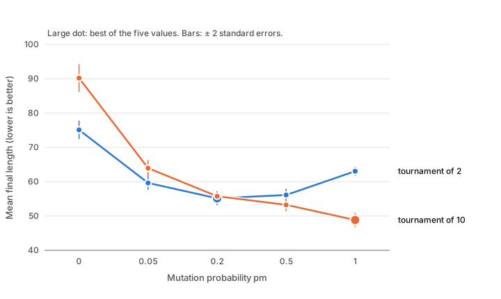
With the same algorithm, the map of 20 destinations, and 30 replicates, we repeated the pm experiment with a tournament of size 2 and one of size 10.
figuras/09-experimentos.py in the book’s repository.
Show the figure data
Mean final length of 30 runs and, in parentheses, the standard error:
| pm | 0 | 0.05 | 0.2 | 0.5 | 1 |
|---|---|---|---|---|---|
| Tournament of 2 | 75.1 (1.3) | 59.6 (1.0) | 55.2 (1.0) | 56.1 (0.9) | 63.1 (0.6) |
| Tournament of 10 | 90.2 (2.0) | 64.0 (1.2) | 55.8 (0.7) | 53.3 (0.9) | 48.8 (1.0) |
With a tournament of 2, the best value of pm among the five is 0.2; raising it to 0.5 does not improve the result, and with pm = 1 the mean rises from 55.2 to 63.1. With a tournament of 10, raising pm improves the result up to the last value, pm = 1. No value of pm is good in itself: it depends on k.
With little mutation, the tournament of 10 is the worst: with pm = 0 it gives 90.2, because such strong selection quickly fills the population with copies (section 9.7). With pm = 1, by contrast, both tournaments keep the population full of different routes, about 30 of 30 until the end. The difference lies in which routes are mutated. With a tournament of 10, the parents are almost always the best individual or very good routes, and mutating all of them amounts to trying, in each generation, about 29 small variations of the best routes: a search around the best found so far. With a tournament of 2, many parents are mediocre routes, and mutating all of them scatters the search.
There is a third piece: replacement. Heavy mutation spoils many offspring, but with an elite the best individual passes unchanged and is never lost (section 8.3), so mistakes are cheap. Without an elite, the best value of pm drops to 0.2, and mutating every individual is a disaster. Mean final length of 30 runs on the map of 20 destinations, with a tournament of 3:
| pm | 0.05 | 0.2 | 0.5 | 1 |
|---|---|---|---|---|
| With one elite individual | 62.6 | 55.4 | 51.6 | 54.8 |
| Without an elite | 64.0 | 55.2 | 57.4 | 81.5 |
The best value of pm therefore depends on selection and on replacement.
There is also interaction between Pc and pm. With pm = 0.05, raising Pc from 0 to 0.6 and 0.9 lowers the mean from 69.0 to 62.6 and 59.9: crossing over helps. With pm = 0.5, the means are 51.2; 51.6; and 53.3, which means that crossover hardly matters. With a lot of mutation and OX, this algorithm hardly needs crossover: it is, above all, a search that mutates and selects many routes at once. In section 9.10 we will see that the same does not happen with a crossover that preserves what matters in the traveling salesman problem.
Show the data on the effect of Pc
Mean final length of 30 runs and, in parentheses, the standard error, on the map of 20 destinations with a tournament of 3:
| Pc | 0 | 0.6 | 0.9 |
|---|---|---|---|
| pm = 0.05 | 69.0 (1.2) | 62.6 (0.9) | 59.9 (1.0) |
| pm = 0.5 | 51.2 (0.9) | 51.6 (1.0) | 53.3 (1.1) |
The practical consequence is that combinations must be tested. A full factorial design tests all combinations of the values (“levels”) of each parameter (“factor”). With 4 parameters and 5 levels each, there are 5^4 = 625 combinations (Eiben & Smith, 2015, p. 123), and with 30 replicates each, 18 750 runs. Schaffer and his colleagues carried out such a design with 6 population sizes, 10 values of Pc, 7 of pm, and one or two crossover points: 840 combinations with 10 replicates each. That came to 8400 runs, which took about a year and a half of computing time on the computers of 1989; among their test problems was a traveling salesman problem with 30 cities (Schaffer et al., 1989, p. 53). It is a high cost, and combinations are cut down with designs such as the Latin hypercube, or bad configurations are discarded early with racing algorithms (Eiben & Smith, 2015, p. 129; Talbi, 2009, p. 55).
You start with a tournament of 2 and tune pm with the data in figure 9.4. Then, with that pm, you try a tournament of 10 in case it improves things. Which combination do you keep? Which is the best one in the figure? How much longer is the mean route of the one you choose?
Show the solution
With a tournament of 2, the best pm among the five is 0.2 (55.2). With that pm, the tournament of 10 gives 55.8: it does not improve, and we keep the tournament of 2. But the best combination in the figure is a tournament of 10 with pm = 1, at 48.8. The route we chose is 13% longer (55.2/48.8 ≈ 1.13). Tuning one at a time has left us at a local optimum of the tuning itself. To find the best, combinations must be tested.9.10 Operators, Representation, and Locality AdvancedA
This section requires sections 6.10 and 7.9.
We have tuned Pc, pm, and k with EvoTraveller’s operators, OX crossover and swap mutation. Does the value of the parameters matter as much as the choice of operators?
In the traveling salesman problem, the length of a route depends only on which cities are neighbors: on its edges (Talbi, 2009, p. 92). A good operator for this problem should preserve most of the parents’ edges. This is the locality from section 7.10: a small change in the chromosome should produce a small change in the solution (Talbi, 2009, p. 209). In crossover, it is the heritability from section 6.1: offspring should resemble their parents in what made them good. What each operator preserves depends on how the chromosome is read. OX preserves above all the relative order, and ERX the adjacencies, which are the edges (section 6.10). Swap mutation breaks up to four edges, and inversion of a stretch only two (section 7.9).
We measured this on the map of 20 destinations, on 60 good, distinct routes with a mean length of 46.8. They are local optima of a local search with inversions, starting from random routes. Each route, including the departure from and return to the origin, has 21 edges. Each mutation was applied 50 times to each route, and each crossover 20 times to each of 30 pairs:
| Operator | Edges kept (of 21) | Mean change in length |
|---|---|---|
| Swap mutation | 17.4 | 32.7% |
| Inversion mutation | 19.0 | 18.3% |
| Crossover | Child’s edges that come from a parent | Child’s length relative to the better parent |
|---|---|---|
| OX | 86% | +24% |
| PMX | 88% | +24% |
| CX | 81% | +42% |
| ERX | 96% | +11% |
Inversion and ERX are the most local operators for the traveling salesman problem: they break fewer edges, and their results are closer in length to the starting routes. Does this show in the genetic algorithm? We repeated it with each combination of crossover and mutation, with the rest of the parameters as in figure 9.1 (Pc = 0.6 except in the row without crossover):
| Crossover | Swap, pm = 0.05 | Swap, pm = 0.5 | Inversion, pm = 0.05 | Inversion, pm = 0.5 |
|---|---|---|---|---|
| No crossover | 69.0 | 51.2 | 60.0 | 43.0 |
| OX | 62.6 | 51.6 | 53.9 | 42.5 |
| PMX | 65.1 | 48.9 | 55.2 | 43.0 |
| CX | 66.7 | 52.6 | 57.9 | 43.9 |
| ERX | 53.9 | 43.3 | 53.1 | 42.4 |
Show all the data
Mean final length of 30 runs and, in parentheses, the standard error:
| Mutation and pm | No crossover | OX | PMX | CX | ERX |
|---|---|---|---|---|---|
| Swap, 0.05 | 69.0 (1.2) | 62.6 (0.9) | 65.1 (0.9) | 66.7 (1.0) | 53.9 (0.9) |
| Swap, 0.2 | 57.3 (0.9) | 55.4 (1.0) | 56.7 (0.7) | 55.5 (1.0) | 48.0 (0.7) |
| Swap, 0.5 | 51.2 (0.9) | 51.6 (1.0) | 48.9 (1.0) | 52.6 (0.8) | 43.3 (0.6) |
| Swap, 1 | 53.6 (0.9) | 54.8 (1.0) | 52.8 (0.8) | 52.5 (0.9) | 52.2 (0.7) |
| Inversion, 0.05 | 60.0 (0.9) | 53.9 (0.8) | 55.2 (1.0) | 57.9 (0.7) | 53.1 (0.9) |
| Inversion, 0.2 | 45.9 (0.6) | 44.7 (0.5) | 45.0 (0.6) | 46.3 (0.6) | 44.6 (0.5) |
| Inversion, 0.5 | 43.0 (0.4) | 42.5 (0.4) | 43.0 (0.4) | 43.9 (0.5) | 42.4 (0.4) |
| Inversion, 1 | 45.5 (0.5) | 48.8 (0.6) | 46.4 (0.4) | 49.5 (0.5) | 45.7 (0.5) |
With swap mutation, ERX improves the mean for every value of pm tested, and the best mean falls from 51.6 with OX to 43.3 with ERX, 16% less. No value of pm achieves that with OX. The best route we have found for this map, by repeating the local search with inversions from 300 random routes, has length 40.68. With ERX, moreover, crossover does help even when there is a lot of mutation: with pm = 0.5, the mean falls from 51.2 without crossover to 43.3. What we saw in section 9.9, that with a lot of mutation crossover hardly matters, was true for OX, which does not preserve edges well, not for every crossover.
With inversion, on the other hand, the mutation already preserves the edges, and the crossovers resemble one another: with pm = 0.5, all of them end between 42.4 and 43.9, and without crossover, at 43.0. Crossover helps mainly when mutation is scarce (with pm = 0.05, from 60.0 without crossover to 53.1 with ERX). With both kinds of mutation, the best of the pm values tested is still 0.5 (with CX and swap mutation, 0.5 and 1 tie). For reference, a hill climber that starts from the best of 30 random routes and in each generation tries 29 mutations of the best route, keeping the best one if it is no worse, makes the same number of evaluations and reaches 54.9 with swaps and 42.2 with inversions.
The conclusion is that parameters are tuned after choosing a representation and operators that preserve what matters in the problem. Fine-tuning pm does not make up for operators with poor locality. In EvoTraveller the operators are fixed (OX and swap); the “Compare operators” screens in crossover-ga and mutation-ga show what each one preserves (sections 6.10 and 7.9).
With OX and swap mutation, our starting point, the mean is 62.6 with pm = 0.05. With the data in this section, which improves the mean more: raising pm to 0.5, or replacing OX with ERX without touching pm? And doing both? Why does it make almost no difference which crossover is used with inversion and pm = 0.5?
Show the solution
Raising pm to 0.5 lowers the mean to 51.6, 18% less. Replacing OX with ERX with pm = 0.05 lowers it to 53.9, 14% less. Both at once, to 43.3, 31% less, within 6% of the best known route (40.68). With inversion, the mutation itself performs a local search that respects the edges: the algorithm reaches about 42–44 with any crossover when pm = 0.5, and the choice of crossover is no longer decisive.9.11 Further Reading Further reading+
Prior tuning with another algorithm. Because parameter tuning is an optimization problem, it can be solved with a genetic algorithm. Grefenstette did so with a “meta-level” genetic algorithm whose population consisted of 50 parameter sets, and each individual encoded the population size, Pc, pm, the generation gap, a scaling technique, and whether elitism was used; its fitness depended on the performance of a genetic algorithm with those parameters (Grefenstette, 1986, pp. 124–125; Mitchell, 1996/1998, Section 5.6). In this way he evaluated 1000 configurations, each with five test functions. Because a single run depends on chance, he retested the 20 best with five different seeds before choosing the winner (Grefenstette, 1986, p. 125). Talbi presents this as a two-level scheme: the upper level optimizes the parameters, and evaluating each set requires running the lower-level metaheuristic on the real problem, which makes it very expensive (Talbi, 2009, pp. 55–56). Eiben and Smith call the quality of a parameter set its utility, to distinguish it from the fitness of a solution. Unlike fitness, utility always depends on chance, because it is measured with runs of a stochastic algorithm (Eiben & Smith, 2015, pp. 122–123). Today there are specific tuning methods, such as F-race, SPO, or REVAC (Eiben & Smith, 2015, p. 124).
Controlling the parameters during the run. The best value of a parameter can change during the search: for example, more mutation may be useful when the population has lost diversity. Eiben et al. (1999, pp. 124, 129) distinguish between tuning the parameters before the run, after which they do not change, and controlling them during it. They classify control into three forms, also covered by Talbi: dynamic or deterministic updating, which does not look at how the search is going (for example, a value that decreases with the generations); adaptive updating, which changes it according to progress; and self-adaptive updating, in which the parameters are encoded in the chromosome and evolve with the solutions (Eiben et al., 1999, p. 129; Talbi, 2009, p. 56). Mitchell notes that many researchers consider real-time adjustment the most promising approach, and that in evolution strategies the mutation rate is encoded in the chromosome (Mitchell, 1996/1998, Section 5.6).
Robustness and overfitting. The word robustness is used in three senses: an algorithm can be robust to chance, if it gives similar results with different seeds (section 9.3); to problems, if it works well on different instances; or to its parameters, if it works well with different values (Eiben & Smith, 2015, pp. 126–127). If the parameters are tuned on some instances and the algorithm is evaluated on the same ones, the result is too favorable: the values are excellent for those instances and much worse for others, and robustness to unknown instances is lost (Talbi, 2009, p. 63). This can also happen to a whole community that always compares its algorithms on the same test functions: it ends up with algorithms that are better and better for those functions, but not for other problems (Eiben & Smith, 2015, p. 159). That is why tuning instances are kept separate from evaluation instances. But if several configurations are compared on the evaluation instances to keep the best one, those instances are also being used to choose, and the winner’s figure is again optimistic. To estimate the quality of the chosen configuration without cheating, three groups are used: some cases for tuning, others for validation to choose, and others for testing, which are kept until the end and used only once, with the configuration already chosen (Hastie et al., 2009, Section 7.2, p. 222). We will do this in section 10.6.
Statistical tests. The confidence interval in section 9.8 is a simple way to compare. Talbi mentions other tests: Student’s t-test for paired data when they are approximately normal, and the Wilcoxon, permutation, and Mann–Whitney tests when they are not (Talbi, 2009, pp. 63–64). To compare more than two configurations, one begins with an analysis of variance (ANOVA), which also makes it possible to study the interaction of two parameters, and if the data are not normal, rank-based tests are advisable (Eiben & Smith, 2015, pp. 157–158). The success rate is also used: the ratio between the runs that reach a reference solution (the optimum, the best known solution, or another fixed in advance) and the total number of runs (Talbi, 2009, p. 64). This is what we did in section 8.5: without an elite, 17 of 30 runs reached the optimum, and with an elite, all 30. Together with the mean best fitness (the mean, across runs, of the best fitness at the end, which is what we have measured in this chapter with the length of the best route) and the average number of evaluations to a solution (counting only the runs that reach it), it forms the three most widely used measures (Eiben & Smith, 2015, pp. 126, 151–153). The first two are measured with a computing limit fixed in advance, and if the limit changes, the winner may change: an algorithm that improves quickly and then stagnates wins with little time, and another that is slower but steady wins with a lot (Eiben & Smith, 2015, p. 152).