11 Recap
Tools: the portal, which brings together all the tools from the previous chapters. This is a review chapter: almost all the activities are pencil-and-paper exercises.
After completing the basic path through this chapter, you will be able to:
- list the nine design decisions of a genetic algorithm and, for each one, the starting option from the basic path;
- choose the representation for a new problem and, with it, the initialization, crossover, and mutation;
- recognize in a design the mistakes revealed by the book’s counterexamples, and correct them;
- decide whether a genetic algorithm, or another metaheuristic, is a reasonable option for a problem;
- design a complete genetic algorithm for a new problem and plan how to tune it according to the time available;
- recognize where genetic algorithms are used and how they are combined with other methods, and name the main topics that this book leaves out.
11.1 The Nine Decisions at a Glance BasicB
You have seen each piece of a genetic algorithm separately. What has to be decided to assemble the whole thing, and where is the best place to start?
In section 2.8 we gathered the design into nine decisions. The table lists them again, now with the starting option we saw in the basic path of each chapter. It is a starting point, not a recipe: each option has alternatives and counterexamples, and the chapters explain when it is better to change it.
| Decision | Question | Starting option | Where |
|---|---|---|---|
| 1. Representation | How is a solution written? | The most natural one for the problem: bits for yes-or-no decisions, integers for choosing among options, a permutation for ordering, and real numbers for continuous variables | 3 |
| 2. Initialization | What population do we start with? | Random and uniform; permutations, by shuffling with Fisher–Yates. It must be diverse, not good | 4.1–4.3 |
| 3. Genotype and phenotype | How do we go from the chromosome to the solution? | Direct in integer, real, and permutation representations; in a yes-or-no binary representation, each bit indicates whether the element is included; for numerical variables, read each group of bits as an integer and, if appropriate, map it to the interval | 3.1–3.6 |
| 4. Fitness | How do we measure how good a solution is? | From the objective function. If a cost is minimized, it must be transformed for the roulette wheel; constraints that the representation does not absorb are handled with a penalty | 4.5–4.7 |
| 5. Mutation | How are small changes introduced? | Bit-flip; random resetting or creep in the integer representation; Gaussian in the real one; swap, insertion, or inversion in the permutation. With a small pm | 7 |
| 6. Crossover | How are two parents combined? | One-point, two-point, or uniform in binary and integer representations; uniform or arithmetic in the real one; OX, PMX, or CX in the permutation | 6 |
| 7. Selection | Who reproduces? | Tournament, which depends only on the ranking; roulette wheel, with care for the scale of the fitness | 5 |
| 8. Replacement | Who passes into the next generation? | Generational with a small elite | 8.2–8.3 |
| 9. Stopping | When does the run end? | When the optimum is reached, if it is known; when the resources run out; or after several generations without improvement | 8.6 |
In addition to the decisions, there are the parameters: the population size N and the crossover and mutation probabilities Pc and pm. Classic studies used populations of 20 to 100 individuals, Pc between 0.6 and 0.95, and pm between 0.001 and 0.01 per bit, but those values were obtained with particular problems, and there is no set of values that is best for all of them (section 9.5). That is why parameters are tuned with cases similar to the real one and compared using several runs (chapter 9). And before tuning them, we need to know how much time there is for the search, which depends on the horizon of the decision (section 9.6). In a strategic problem, which is solved once and whose consequences last for years, a lot can be spent on the search: large populations, many generations, and several runs to keep the best one. In an operational problem, which is solved very frequently, sometimes in real time, the evaluation budget is small, and a fast configuration that rarely fails is preferable. Tactical problems, in the medium term, lie between the two (Eiben & Smith, 2015, pp. 147–149; Talbi, 2009, pp. 33–34).
The order of the table is the order of design. Representation comes first, because fitness is calculated on the decoded solution, and crossover and mutation have to be designed for the chromosome (section 2.8). Selection, replacement, and stopping, on the other hand, do not depend on the representation: they look at fitness (and stopping also at the computational budget spent), so they work the same for any representation.
A paper says: “We used a genetic algorithm with a population of 100 individuals, a crossover probability of 0.8, and a mutation probability of 0.01, for 200 generations.” With this information, could you repeat the experiment? Which decisions are missing?
Show the solution
It could not be repeated. Only the parameters and one of the nine decisions are known: stopping (200 generations). What is missing:
- the representation and the decoding: how each solution is written;
- the initialization;
- the fitness: how to go from the objective to fitness and what is done with the constraints;
- which crossover and which mutation. Moreover, “0.01” does not say whether it is the probability that each gene mutates or that each individual does, and these are not the same (section 9.2);
- the selection, with its parameters, such as the tournament size;
- the replacement: whether there is an elite and how large it is.
11.2 A Map by Representation BasicB
The previous table says what has to be decided. But once the representation has been chosen, what options remain for the other decisions?
First, it is worth recalling how the representation is chosen. The starting question is what a solution to the problem is: a subset of elements, an option for each element, an order, or a set of numbers. Each answer points to one of the book’s four representations, as figure 11.1 summarizes (Talbi, 2009, pp. 36–37). It is a guide, not a rule: the same problem sometimes admits another representation, such as the knapsack written with a permutation and a decoder (section 3.10) or the traveling salesman problem written with random keys (section 3.13). Nor is it exclusive to genetic algorithms: any metaheuristic has to decide how a solution is written. What is specific to the genetic algorithm is the distinction between the chromosome, which crossover and mutation manipulate, and the solution that is evaluated (section 3.1).
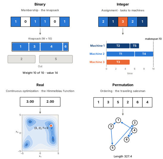
figuras/11-tipos-de-representacion.py in the book’s repository.
Almost everything that depends on the representation comes down to initialization, decoding, and the two variation operators. For each of the book’s four representations, the table brings together what we saw in the basic path and, in the last row, the alternatives from the advanced sections.
| Binary | Integer | Real | Permutation | |
|---|---|---|---|---|
| What for | Yes-or-no decisions (the knapsack, which projects are funded) and numbers in an interval | Choosing an option for each element (assigning tasks to machines, time slots to exams, or a site to each warehouse) | Continuous variables (the Himmelblau function, fitting the parameters of a model) | Ordering (the traveling salesman, job sequencing, the order of the stops on a delivery route) |
| Decode | Yes or no: each bit indicates whether the element is included. For numerical variables: bits → integer → interval, with precision \Delta = (b-a)/(2^k-1) (3.2–3.3) | Direct: the gene is the option (3.4) | None: the chromosome is the point (3.6) | The order of the permutation; in the traveling salesman problem, plus the origin at the beginning and the end (3.5) |
| Initialize | Each bit 0 or 1 with equal probability (4.1) | Each gene uniform over its range | Each gene uniform over its interval | Shuffle with Fisher–Yates (4.2) |
| Validity and feasibility | Every string is valid but may not be feasible (an overweight knapsack) (3.7) | Valid if each gene is within its range | Every vector is valid; outside the interval, the solution is not feasible (3.11) | Each element exactly once: the operators must respect this |
| Crossover | One-point, two-point, uniform (6.2–6.3) | The same as for binary | Uniform and arithmetic (6.4) | OX, PMX, and CX (6.6–6.8) |
| Mutation | Bit-flip with pm per gene (7.2) | Random resetting for categories; creep for ordered quantities (7.3) | Gaussian, with step size σ (7.4) | Swap, insertion, and inversion (7.6) |
| Advanced | Gray code (3.8); k-point crossover; single-bit mutation | Circular creep | Quasi-random initialization and Latin hypercube (4.9); BLX-α and SBX; uniform, non-uniform, and polynomial mutation | Variants of OX and CX, and ERX (6.9); scramble mutation (7.8) |
Three ideas run through the table. First, operators are chosen according to the representation, not the other way around. One-point crossover and random resetting work with bits and integers, but they repeat cities if they are applied to a permutation (sections 6.5 and 7.5). Second, within a representation, the right operator depends on what the genes mean. If the gene is a category, such as a machine, random resetting is natural; if it is an ordered quantity, creep gives small changes (section 7.3). Third, a valid chromosome need not be a feasible solution. When the representation does not absorb a constraint, we have to penalize, repair, or reject (sections 3.7 and 4.7).
For each problem, choose the representation, a crossover, and a mutation from the basic path. Is there any constraint that the representation does not absorb?
- A company has an advertising budget and 25 possible ads, each with its price and estimated reach. Which ads should it buy?
- 30 orders have to be distributed among 5 trucks.
- The order in which 10 jobs are processed on a single machine has to be decided so that they are delayed as little as possible.
- The diameter, between 10 and 50 mm, and the wall thickness, between 1 and 5 mm, of a pipe have to be chosen.
Show the solution
| Representation | Crossover | Mutation | Constraint | |
|---|---|---|---|---|
| a) | Binary, one bit per ad (like the knapsack) | One-point, two-point, or uniform | Bit-flip | The budget: a string can exceed it. We must penalize or repair |
| b) | Integer, one gene per order with its truck, from 1 to 5 | One-point, two-point, or uniform | Random resetting: the truck number is a label, not a quantity | If the trucks have a capacity, a truck can be overloaded: penalty |
| c) | Permutation of the 10 jobs | OX, PMX, or CX | Swap, insertion, or inversion | None, if the operators respect the permutation |
| d) | Real, with two genes | Uniform or arithmetic | Gaussian | The intervals: Gaussian mutation can take a gene outside its interval (section 3.11) |
11.3 Common Mistakes BasicB
Throughout the book, several counterexamples have appeared: decisions that seem reasonable but are not. Which ones are worth remembering when designing a genetic algorithm?
| Mistake | What happens | What to do | Where |
|---|---|---|---|
| Seeding without caring about diversity | Selection can concentrate the population around a few solutions | A random initial population; if seeding, a randomized heuristic that gives different solutions | 4.4 |
| Using a cost as fitness with the roulette wheel | The roulette wheel favors the worst, or cannot be built if there are negative values | Transform the cost (C - f, 1/(1+f), the rank) or use the tournament | 4.6 |
| Choosing the penalty weight badly | If λ is small, infeasible solutions win; if it is very large, promising infeasible solutions are lost | Try several weights with similar cases | 4.7 |
| Using the roulette wheel with very similar fitness values | Everyone has almost the same probability: selection stops distinguishing | Tournament, ranking, or scaling | 5.4 |
| Letting only the best reproduce | Truncation reduces diversity very quickly | A selection that gives everyone a chance | 5.5 |
| Applying string operators to a permutation | One-point crossover and random resetting repeat elements | Permutation operators | 6.5, 7.5 |
| Mutating too much | The search becomes random | A small pm, for example 1/L per gene, with L genes | 7.7 |
| Generational replacement without an elite | The best solution can be lost | A small elite | 8.3 |
| Comparing generations across different algorithms | A steady-state generation evaluates one child, and a generational one N | Count evaluations | 4.8, 8.4 |
| Drawing conclusions from a single run | The result depends on the seed | Several replicates, means, and standard deviations | 9.3–9.4 |
| Tuning without thinking about the time available | The chosen configuration does not finish in time in an operational problem, or falls short in a strategic one | Set the budget first according to the horizon of the decision | 9.6 |
| Tuning and evaluating with the same cases | The parameters look better than they are | Choose with some cases (tuning and validation) and estimate the quality with others (test) | 9.5, 10.6 |
Many of the mistakes in the table have the same root: breaking the balance between the two forces of section 1.3, exploitation and exploration from section 1.5. Seeding without preserving variety, truncating, or removing mutation can give too much exploitation, and the population gets stuck; mutating too much or removing the elite means that what has been found can be lost. The others are mistakes of representation, measurement, or planning: a fitness that does not distinguish, an experiment that does not allow conclusions to be drawn, or a budget that does not match the problem.
A team designs a genetic algorithm for a traveling salesman problem with 30 cities:
- Each route is a permutation of the cities.
- The initial population consists of 50 copies of the nearest-neighbor route, each with one random swap.
- Fitness is the length of the route, and parents are chosen with the roulette wheel.
- One-point crossover, with Pc = 0.9.
- Swap mutation, with pm = 0.05 per individual.
- The offspring replace all the parents.
- The run stops after 500 generations.
- To choose between pm = 0.05 and pm = 0.2, they do one run with each value and keep the one that gives the shorter route.
Which decisions are wrong? How would you correct them?
Show the solution
- 2. This is seeding with a heuristic: the 50 routes are almost the same, and the population starts with no diversity (section 4.4). Better: random permutations with Fisher–Yates.
- 3. Length is minimized, but the roulette wheel gives more probability to higher fitness: it would favor the longest routes (section 4.6). It must be transformed, for example with the inverse of the length, as EvoTraveller does, or the tournament must be used.
- 4. One-point crossover gives offspring with repeated cities (section 6.5). OX, PMX, or CX must be used.
- 6. Without an elite, the best route can be lost (section 8.3). The best individual should be passed on unchanged.
- 8. One run per value is not enough: the difference may be due to the seed (section 9.4). The means of several replicates must be compared, on maps similar to the real one.
11.4 Designing for a New Problem BasicB
You have a problem that nobody has given you as an exercise. Where do you start?
First, is it worth it? A genetic algorithm is not the best option for everything. Mitchell reports an intuition shared by many researchers, although it is not a rigorous rule: a genetic algorithm has a good chance of competing with other general methods when the search space is large, is not smooth or does not have a single peak, or is poorly understood, when the fitness is noisy, and when it is enough to find a good-enough solution quickly. On the other hand, if the space is small, it can be searched exhaustively; if it is smooth or has a single peak, a method that climbs the slope is much more efficient; and if the problem is well understood, like the traveling salesman problem, methods that use specific heuristics usually give better results (Mitchell, 1996/1998, Section 5.1). A recent review sums it up in the same way: genetic algorithms are useful above all in large, complex, and poorly understood search spaces, where classic methods, such as enumeration or heuristics, are not suitable (García-Martínez et al., 2025, p. 652). We saw this when estimating the size of a search space (section 1.4) and when combining the genetic algorithm with a local search (section 10.9).
A metaheuristic is a general search method, applicable to almost any optimization problem, that gives satisfactory solutions in a reasonable time, although with no guarantee of finding the optimum; the genetic algorithm is one of them (section 11.6). These three questions (is the space small? is it smooth? are there specific heuristics?) actually apply to any metaheuristic: they decide whether an approximate, general method is needed. A fourth one remains, the one that chooses among them. What is specific to the genetic algorithm is that crossover combines the information of two solutions, whereas many other methods explore the neighborhood of a single one (García-Martínez et al., 2025, p. 629). In general, population-based methods tend to explore the space, and those that transform a single solution, trajectory methods, tend to exploit a region (Talbi, 2009, p. 25). A genetic algorithm makes most sense when combining parts of good solutions yields good solutions, that is, when crossover passes on meaningful pieces (section 6.1), or when it is useful to search with many solutions at once, because there are several peaks or several objectives. Figure 11.2 summarizes the path. It is a guide, not a rule, and often the best thing is to combine both types of method.
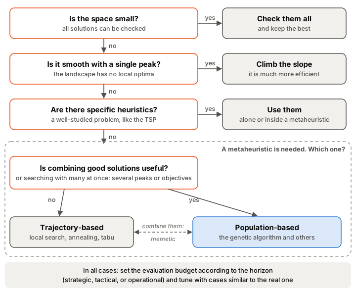
figuras/11-que-metodo.py in the book’s repository.
Then, the design. If the answer is a genetic algorithm, go through the nine decisions in the order of section 11.1:
- Write down a solution: choose the representation with the table in section 11.2 and count how many chromosomes there are.
- Write down the objective and the constraints. Decide which ones the representation absorbs and how you will handle the rest.
- Choose the initialization, crossover, and mutation that correspond to the representation and to the meaning of the genes.
- Choose the selection, the replacement, and the stopping criterion.
- Decide how much time there is for the search, according to the problem’s horizon. Set some starting parameters and tune them with cases similar to the real one, with several replicates per configuration. Check the result on new cases.
- Go over the table of mistakes in section 11.3.
- In Five modules. One shared process., match each module with the decisions in section 11.1. Which decisions do not have a module of their own?
- Scroll down to How they fit into the algorithm and compare the cycle with figure 2.1. Why must the offspring be evaluated before replacement, if replacement compares parents and offspring?
- In Experiment across generations, choose the simulator you would use to check the effect of selection pressure over many generations and the one you would use to tune pm in the traveling salesman problem.
Would you use a genetic algorithm in these cases? Explain your answer.
- Choosing which of 15 projects to fund without exceeding the budget. A computer evaluates a million combinations per second.
- Finding the minimum of a smooth function with a single minimum and a known derivative.
- Tuning six real parameters of a simulation of a factory. Each evaluation takes one minute, gives a noisy result, and there are many local optima. A good configuration is enough.
- Finding a very short route for a traveling salesman problem with 1 000 cities and straight-line distances.
Show the solution
No. With 15 projects there are 2^{15} = 32\,768 combinations, which can all be checked in a few hundredths of a second, and this finds the best one with certainty.
No. A method that climbs (or descends) the slope uses the derivative and reaches the minimum much sooner.
Yes, it is a good candidate. The space is continuous and has many local optima, the fitness is noisy, and a good-enough solution is sufficient. But each evaluation is expensive: the evaluation budget must be counted (section 4.8), and we must decide how to handle the noise (section 4.13).
Not as the only method. The traveling salesman problem is very well studied, and there are specific heuristics that usually work better. If a genetic algorithm is used, the sensible thing is to combine it with a local search, such as 2-opt (section 10.9).
A school has to schedule 40 exams in 8 time slots. Some pairs of exams have students in common and cannot be in the same slot. In addition, because of the rooms available, there can be no more than 6 exams in one slot. The goal is the timetable with the fewest conflicts. A computer evaluates a million timetables per second.
- With 12 exams and 4 slots, would you use a genetic algorithm? And with 40 exams and 8 slots?
- Design a genetic algorithm for the case of 40 exams: the nine decisions and some starting parameters.
- How would you check that the design works before using it on the real timetable?
- Go over your design with the table of mistakes in section 11.3, as step 6 of the procedure asks. Which mistakes does it avoid, and which would you have to watch out for?
Show the solution
With 12 exams and 4 slots there are 4^{12} = 16\,777\,216 timetables: at a million per second, they can all be checked in about 17 seconds. A genetic algorithm is not needed. With 40 exams and 8 slots there are 8^{40} = 2^{120} \approx 1.3 \times 10^{36}, and checking them all would take about 4 \times 10^{22} years. Here it does make sense.
One proposal:
| Decision | Proposal |
|---|---|
| 1. Representation | Integer: 40 genes, one per exam, with its slot, from 1 to 8. Every chromosome is valid but may not be feasible |
| 2. Initialization | Each gene uniform between 1 and 8 |
| 3. Genotype and phenotype | Direct: gene i is the slot of exam i |
| 4. Fitness | Minimize the number of pairs of exams with students in common in the same slot plus λ for each exam over the limit in a slot. The value 0 is a conflict-free timetable that fits in the rooms |
| 5. Mutation | Random resetting: as far as conflicts are concerned, the slot is a label, and there is no reason to prefer nearby slots. With pm = 1/40 per gene |
| 6. Crossover | Uniform: the numbering of the exams is arbitrary, so there is no reason to keep neighboring genes together |
| 7. Selection | Binary tournament: it depends only on the ranking, so there is no need to transform the cost |
| 8. Replacement | Generational with an elite of 1 |
| 9. Stopping | When the fitness reaches 0, when a maximum number of evaluations has been used up, or after many generations without improvement |
Starting parameters: a population of 50 to 100 and Pc = 0.8, within the classic values. Other options are reasonable if they are justified: for example, the roulette wheel with a transformed fitness, or handling capacity with a repair that moves exams out of full slots.
With timetables from previous years, which are cases similar to the real one: try several values of λ, pm, and the tournament size, with 30 replicates per configuration, and compare the means and standard deviations. Then check the chosen configuration on timetables that were not used to tune it (sections 9.5 and 10.6). The timetable is made once per semester and there are days to calculate it, so it is a tactical problem, almost a design problem (section 9.6): a large population and many generations can be afforded, and several runs can be made on the real timetable to keep the best one.
The proposal avoids several mistakes in the table: the initial population is random, without seeding; the tournament needs no transformation of the cost and does not stop distinguishing with similar fitness values; the operators are integer-vector operators, not string operators applied to permutations; pm = 1/40 is small; there is an elite; and in c), replicates are used, along with different cases for choosing the configuration and for estimating its quality. Two things remain to watch: the penalty weight λ, which should be tried with several values, and the budget, which must be set according to the days available. If it is compared with a steady-state version, evaluations must be counted, not generations.
11.5 Genetic Algorithms in Practice BasicB
Outside of exercises, who uses genetic algorithms, for what, and how?
Where they are used. In almost every field. A Scopus search in April 2024 found 71 147 documents with “genetic algorithm” in the title. For about the last fifteen years, more than 3500 have appeared each year, and the fields with the most papers are engineering and computer science, followed by mathematics, physics, materials science, and energy (García-Martínez et al., 2025, pp. 652–653). Engineering problems are often the hardest: they have several objectives, change over time, have many interrelated variables, and have strict constraints (García-Martínez et al., 2025, p. 653). Many resemble those in the book: distributing tasks among machines and sequencing jobs, designing delivery routes, building timetables, or fitting the parameters of a model. They are also used in machine learning: to choose which variables or which data a model uses, to find classification rules, to tune a model’s hyperparameters, or to search for the architecture of a neural network (García-Martínez et al., 2025, pp. 654–655).
How they are used. Almost never alone, and almost never programmed from scratch:
- Combined with other methods. A common use is for the genetic algorithm to find promising regions and for another method to refine them, as local search does in memetic algorithms (section 10.9). They are also combined with mathematical programming, in matheuristics, and with simulation, in simheuristics, when evaluating a solution requires simulating a system under uncertainty, like the factory in exercise 11.4 (García-Martínez et al., 2025, p. 648). Section 11.6 gives more details.
- With a library. The portal’s tools let you follow each step with its code in Python and JavaScript, but this book does not teach how to program a complete genetic algorithm. To do so, besides writing it from scratch, you can use a library. Libraries save work and make it easier to repeat and extend experiments, and if the algorithms being compared are programmed with the same library, the comparison is fairer (Talbi, 2009, p. 67). Some well-known ones in Python are DEAP, for evolutionary algorithms in general (Fortin et al., 2012), PyGAD, for genetic algorithms (Gad, 2024), and pymoo, for multi-objective optimization (Blank & Deb, 2020); in R, the GA package (Scrucca, 2013). With any of them, the nine decisions of section 11.1 remain the same: the library makes them easier, but it does not make them for us.
A team wants to predict the demand for a product with a statistical model. It has 200 candidate variables and wants to choose a subset with which the model predicts well. To evaluate a subset, the model must be fitted and its error measured on data not used to fit it, which takes about 3 seconds.
- What representation would you use? Which problem in the book does it resemble?
- Besides predicting well, a model with few variables is preferred. How could the fitness take this into account?
- Go through the four questions in figure 11.2. Is a genetic algorithm reasonable?
- How many evaluations fit into one night of computing, of 8 hours?
- Is it enough that the data used to compare subsets have not been used to fit the model’s coefficients? How would you measure the final error of the choice?
Show the solution
Binary, with one bit per variable: 1 if it enters the model and 0 if not. It is like the knapsack: each item is a variable (section 3.2). One-point, two-point, or uniform crossover and bit-flip mutation all work.
For example, minimize the error plus λ for each variable used, a penalty like the one in section 4.7. Because it is minimized, the tournament or a transformation of the fitness is advisable. Another option is to treat it as a problem with two objectives, error and number of variables (section 11.6).
The space is not small: there are 2^{200} \approx 1.6 \times 10^{60} subsets. It is not smooth, because removing or adding one variable can change the error a lot, and the measured error depends on which data are set aside to measure it, so it is somewhat noisy. There are specific heuristics, such as stepwise selection, which adds or removes variables one at a time, but they do not guarantee the best subset. And combining makes sense: if two subsets predict well, each may have useful variables that crossover brings together in one child. Yes, it is reasonable, although it should be compared with stepwise selection.
8 \times 3600 / 3 = 9600 evaluations, for example about 95 generations of 100 individuals. The budget is tight: evaluations must be counted (section 4.8), and a small population may be advisable. Choosing the variables is done once, when building the model, so it is a design problem: if there are more nights, several runs can be made.
No. The data used to compare subsets are validation data: they also help choose the model, even though they do not fit its coefficients. Once the variables are fixed, their final error should be measured on other test data that played no part in that choice. It is the same separation we made with the maps in section 10.6 (Hastie et al., 2009, Section 7.2, p. 222).
What we have not covered. This book covers the basic genetic algorithm, with a single objective and a single population. It leaves out, among other things, optimization with several objectives, populations divided into islands, hybrid methods, and other metaheuristics. Section 11.6 introduces them briefly, with further reading; they may be covered in more detail in future editions.
Summary
- Designing a genetic algorithm means making nine decisions, starting with the representation, and setting parameters that are tuned according to the time available, which depends on the horizon of the decision, with cases similar to the real one and several replicates.
- The representation determines the initialization, the decoding, and the operators. Selection, replacement, and stopping do not depend on it and work for any representation.
- Many of the common mistakes break the balance between exploration and exploitation (seeding, truncating, mutating too much, removing the elite) or prevent good measurement (a fitness that does not distinguish, a single run).
- A genetic algorithm is appropriate when the space is large and difficult, a good solution is enough, and combining solutions makes sense; if the space is small, smooth, or very well understood, there are usually better methods, and trajectory metaheuristics are the other major alternative.
- Genetic algorithms are used in many fields, from engineering to machine learning, almost always combined with other methods and programmed with a library. Left out of this edition are multi-objective optimization, niching, island populations, hybrids, other metaheuristics, and theory.
This is the end of the basic path. The activity index gathers the examples and exercises so that you can practice them again.
11.6 What Is Left Out Further reading+
An introductory book has to make choices. These are the most important topics left out of this edition. Some of them have already appeared in the further reading of earlier chapters.
Several Objectives
Many real problems have several conflicting objectives: when designing a product, we want at the same time to reduce its cost, improve its quality, and reduce its environmental impact. In these problems, the terms multi-objective and multicriteria are used as synonyms (Talbi, 2009, p. 308). There is no single solution better than all the others, but a set of Pareto optima: solutions in which one objective cannot be improved without worsening another. With a metaheuristic, the aim is to approximate that set with two properties: the solutions should be close to the true Pareto front and spread uniformly along it. The final choice among them is made by the decision maker (Talbi, 2009, pp. 308–309).
In section 4.14 we saw dominance, fronts, and the drawback of the weighted sum. A multi-objective algorithm adds three components to the design: a fitness assignment that turns the vector of objectives into a number, by aggregation, by separate criteria, by dominance, or with quality indicators; a mechanism that preserves diversity along the front; and a form of elitism that keeps the best solutions found (Talbi, 2009, p. 323). Population-based algorithms fit well, because they can find many Pareto optima in a single run (Talbi, 2009, p. 337). The “Several objectives” screen in initialization-and-evaluation-ga is a first way in.
The first genetic algorithm with several objectives was VEGA, by Schaffer (1985), which filled each part of the parent pool by selecting with a different objective. Goldberg (1989, p. 201) proposed assigning fitness by non-dominated fronts, and from the idea of selecting by dominance came MOGA, which scores each individual according to how many individuals dominate it (Fonseca & Fleming, 1993), NSGA (Srinivas & Deb, 1994), and NPGA (Horn et al., 1994). A second generation added elitism: SPEA (Zitzler & Thiele, 1999), which was tested precisely on multi-objective knapsacks, SPEA2 (Talbi, 2009, p. 337; Zitzler et al., 2001), and NSGA-II (Deb et al., 2002), the best known. NSGA-II sorts the population into non-dominated fronts and, within each front, prefers the most isolated solutions according to their crowding distance. In each generation, it pools parents and offspring and keeps the better half, and it chooses parents with a binary tournament that compares the front first and, in case of a tie, the distance (Talbi, 2009, p. 346). Other ideas followed: decomposing the problem into many single-objective subproblems, as in MOEA/D (Zhang & Li, 2007); choosing survivors with an indicator of front quality, such as the hypervolume in SMS-EMOA (Beume et al., 2007); or guiding the search with reference points when there are more than three objectives, as in NSGA-III (Deb & Jain, 2014).
For further study, there are the textbooks by Deb (2001) and Coello Coello et al. (2007) and several reviews: the classic one by Coello Coello (1999), the one by Zhou et al. (2011) on the state of the art, the one by Li et al. (2015) on many-objective problems, the one by Falcón-Cardona & Coello Coello (2020) on indicator-based algorithms, and the one by Liang et al. (2023) on problems with several objectives and constraints, such as a knapsack with a capacity.
Variants of the Algorithm
Niching and speciation. The genetic algorithm in this book tends to drive the whole population to a single peak. To spread it across several peaks, De Jong proposed crowding, in which each child replaces the most similar of a few individuals taken at random (section 8.9). Goldberg and Richardson proposed fitness sharing: the fitness of each individual decreases the more similar individuals it has around it, so that being different is rewarded and the population can spread across several peaks. Crossover has also been restricted, allowing it only between similar individuals so that “species” form, or forbidding it in order to maintain diversity (Mitchell, 1996/1998, Section 5.5). Sharing divides the fitness of each individual by its number of neighbors within a radius σ, weighted by their distance (Talbi, 2009, p. 344).
Structured and parallel populations. In this book’s algorithm, any individual can be crossed with any other. In the island model, the population is divided into subpopulations that evolve separately, each possibly with its own parameters or operators, and from time to time they exchange some individuals (migration). The goal is to delay the convergence of the whole population and encourage diversity. In the cellular model, each individual occupies a cell of a grid, and selection takes place only among its neighbors, so the selection pressure is lower (Talbi, 2009, pp. 468–469). Both models also make it possible to distribute the work across several processors.
Hybrid algorithms. Combining the genetic algorithm with a local search gives memetic algorithms (section 10.9). It is also combined with exact mathematical programming methods, with constraint programming, and with machine learning techniques (Talbi, 2009, Chapter 5). To sort out so many combinations, García-Martínez et al. (2025, pp. 648–649), building on the classifications of Talbi and of Raidl, cross two questions. The first is whether the methods collaborate as black boxes that only exchange solutions or parameters (collaborative) or whether one goes inside the other, as one of its parts (integrative). The second is whether they work at the same time (teamwork) or one after the other, so that what one returns is the starting point of the next (relay). A genetic algorithm that explores and, when it finishes, passes its best solutions to a local search is collaborative and relay; a memetic algorithm, which applies local search to the individuals in each generation, is integrative and teamwork (García-Martínez et al., 2025, p. 650). The combination with mathematical programming methods is called a matheuristic, and with simulation, a simheuristic: the simulation evaluates the solutions in a system under uncertainty, and the metaheuristic searches for them (García-Martínez et al., 2025, p. 648).
Changing problems. In dynamic optimization, the objective function changes over time: in a routing problem, new customers may appear during the search. The algorithm has to detect the change and track the optimum, which also moves (Talbi, 2009, p. 16). This is different from the noisy fitness of section 4.13, in which the optimum does not change, but each evaluation measures it with error. In coevolution, several populations evolve at the same time, and the fitness of each depends on the others, like a predator and its prey (Talbi, 2009, p. 228). Something similar happens in evolutionary game theory, in which the fitness of a strategy depends on the other strategies in the population (section 1.7).
Other Metaheuristics
A genetic algorithm is a metaheuristic: a general search method that can be applied to almost any optimization problem and gives satisfactory solutions in a reasonable time, although with no guarantee of finding the optimum (Blum & Roli, 2003, pp. 269–271). The term first appeared in a paper by Glover on tabu search (Glover, 1986, p. 541). There are many others, and a simple way to classify them is by the number of solutions they work with: a population, or a single solution that moves through the space, a trajectory (Blum & Roli, 2003, p. 272). Figure 11.3 places the best-known ones between the two extremes of section 1.5: random search, which only explores, and the local search that always moves to the best neighbor, which only exploits.
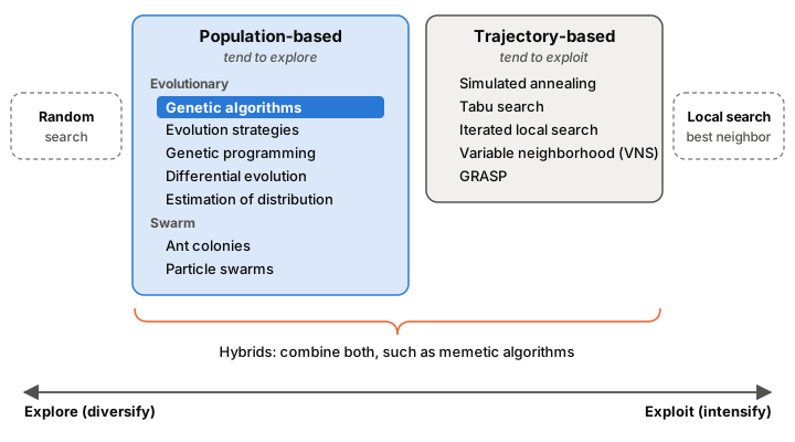
figuras/11-metaheuristicas.py in the book’s repository.
Population-based. Genetic algorithms are one of the families of evolutionary computation (section 2.11), and there are other widely used population-based metaheuristics:
- Evolution strategies. They work with real vectors and Gaussian mutation, and in them each individual can carry its own step sizes, which also evolve (section 7.10). One of their variants, CMA-ES, also adapts the covariance matrix of the mutation, that is, its shape and not just its size (Hansen & Ostermeier, 2001).
- Genetic programming. It evolves programs, represented as trees (Koza, 1992).
- Differential evolution. For continuous problems, it creates new individuals by perturbing those in the population with differences between other individuals (Storn & Price, 1997).
- Estimation of distribution algorithms. They replace crossover and mutation with a probability model that is estimated from the best individuals and from which new ones are sampled (Mühlenbein & Paaß, 1996).
- Swarm intelligence. It is inspired by the collective behavior of animals. Ant colony methods were proposed for combinatorial problems, starting with the traveling salesman problem (Dorigo et al., 1996), and particle swarms for continuous problems (Kennedy & Eberhart, 1995).
Trajectory-based. They transform a single solution, which moves from one neighbor to another (section 2.1). The local search that always moves to the best neighbor stops at the first local optimum (section 1.4), and these methods are ways of escaping from it: sometimes accepting worse neighbors, changing the neighborhood, or starting again from other solutions (Blum & Roli, 2003, pp. 270, 272):
- Simulated annealing. It tries a random neighbor. If it is better, it accepts it; if it is worse, it accepts it with a probability that depends on how much worse it is and on a parameter, the temperature, which decreases little by little, as when a metal is cooled (Kirkpatrick et al., 1983).
- Tabu search. It moves to the best neighbor even if it is worse than the current solution and, to avoid going back, it stores the recent moves in a memory, the tabu list, and forbids undoing them for a while (Glover, 1986, p. 541).
- Iterated local search. When local search reaches a local optimum, it perturbs it, applies local search again, and decides whether to continue from the new optimum or return to the previous one (Lourenço et al., 2003).
- Variable neighborhood search (VNS). It changes the neighborhood, because a local optimum for one neighborhood may not be one for another (Mladenović & Hansen, 1997).
- GRASP. It repeats two steps: it builds a solution with a randomized greedy heuristic, like the one for the knapsack in section 4.4, and improves it with a local search (Feo & Resende, 1995).
In Spanish, Bautista-Valhondo (2020) devotes chapters to local search, GRASP, simulated annealing, and tabu search, as well as to genetic algorithms.
Theory and Parameters
Why does it work? The classic theory, Holland’s theory of schemata and building blocks, appeared briefly in sections 2.11 and 6.11. It does not fully describe the behavior of a genetic algorithm, and other approaches have been developed, such as exact mathematical models and those based on statistical mechanics or on population genetics (Mitchell, 1996/1998, Chapter 6).
No algorithm is best for everything. The no free lunch theorem shows that, under certain conditions, averaged over all possible problems, all optimization algorithms perform the same, random search included: if A is better than B on some problems, B is better than A on others (Wolpert & Macready, 1997). Asking whether one algorithm is better than another only makes sense for a class of problems or instances (Talbi, 2009, p. 103). This is the underlying reason for tuning with cases similar to the real one (section 9.5). It also explains why there are so many crossovers and mutations designed for particular problems: a genetic algorithm works well to the extent that its components, above all the operators, exploit what is known about the problem (García-Martínez et al., 2025, p. 634).
Self-adjusting parameters. Parameters can change during the run, according to a fixed schedule, according to the progress of the search, or encoded in the chromosome itself (section 9.11). Mitchell pointed to this as one of the most promising directions: natural evolution also adapts its own parameters (Mitchell, 1996/1998, Chapter 6).
Further Reading
Eiben & Smith (2015) is a complete textbook on evolutionary computation, and García-Martínez et al. (2025), a brief, recent review of genetic algorithms, from their design to diversity, hybrids, and applications. Their chapter is part of the Handbook of Heuristics, which devotes other chapters to evolutionary algorithms, memetic algorithms, and multi-objective optimization (García-Martínez et al., 2025, p. 655). Talbi (2009) devotes entire chapters to multi-objective optimization (Chapter 4), hybrid algorithms (Chapter 5), and parallel algorithms (Chapter 6). And the last chapter of Mitchell (1996/1998) lists the open questions she saw in the field, such as incorporating ecological interactions between individuals, more mechanisms from genetics, development, and learning, adaptive encodings, and evolving parameters.