8 Replacement and Stopping
Tools: selection-ga, available through the portal.
After completing the basic path through this chapter, you will be able to:
- explain what replacement decides and distinguish generational replacement from steady-state replacement;
- form the next generation by hand with and without an elite, and predict whether the best solution is kept;
- explain what elitism gains and what it risks;
- list the usual stopping criteria and choose one depending on whether the optimum is known and on the resources available;
- read a best-fitness curve and point out where each criterion would stop.
8.1 Who Moves On to the Next Generation? BasicB
We now have the current population and offspring created by crossover and mutation from the parents chosen by selection. Whom do we keep?
In each generation, a genetic algorithm selects parents (chapter 5), crosses them over (chapter 6), and mutates the offspring (chapter 7). What remains is to decide which individuals form the population of the next generation: the offspring, the parents, or a mix of both. This decision is replacement, also called survivor selection: parent selection decides who reproduces, and replacement decides who stays in the population (Talbi, 2009, p. 221). Because the population size is usually constant, if offspring come in, the same number of individuals must leave.
There are two basic strategies (Mitchell, 1996/1998, Section 5.4; Talbi, 2009, p. 221):
- Generational replacement. The offspring replace the entire population of parents. This is the replacement used in Holland’s canonical genetic algorithm and the most widespread one.
- Steady-state replacement. At each step, only one or a few offspring come in, replacing the same number of population members; the rest remain unchanged.
After replacement, the cycle starts again (section 2.2) until a stopping criterion is met. We discuss stopping in section 8.6.
Notation. We follow the tool’s notation. In this chapter, we call all individuals in the current population parents, whether or not selection chose them. They are A, B, C, …, and their number is μ (mu), the population size, which other chapters call N; the offspring are a, b, c, …, and their number is λ (lambda). In chapter 5 we talked about drawing “with replacement” in the sense of returning an individual so that it can be drawn again; in this chapter, replacement means substituting some individuals in the population with others.
In generational replacement, all the offspring replace all the parents. Can the population’s best fitness be worse in the next generation than in the current one? And its mean fitness? Write down your prediction: you will check it in example 8.2.
8.2 Generational Replacement BasicB
If the offspring replace all the parents, what happens to the best parent?
In generational replacement, as many offspring are created as there are parents (\lambda = \mu), and the next generation consists of the offspring alone (Talbi, 2009, p. 221). It is simple, and each generation is a new population. But nothing guarantees that any offspring is as good as the best parent. A good individual can be lost because selection does not choose it or because crossover or mutation destroys what made it good (Mitchell, 1996/1998, Section 5.4).
Data. Six parents and six offspring, already created by crossover and mutation:
| Parent | A | B | C | D | E | F |
|---|---|---|---|---|---|---|
| Fitness | 12 | 30 | 5 | 21 | 9 | 17 |
| Offspring | a | b | c | d | e | f |
|---|---|---|---|---|---|---|
| Fitness | 25 | 3 | 18 | 9 | 14 | 7 |
The screen is called “Generational with elitism”; with an Elite size e of 0, it is pure generational replacement.
Predict. Who forms the next generation? How do the best fitness and the mean fitness change?
Open: generational replacement, e = 0
Show the result
The next generation is a b c d e f: all 6 offspring survive and no parent does. The best fitness falls from 30 to 25, because B has no equally good replacement, and the mean falls from 15.7 to 12.7. This answers exercise 8.1: with pure generational replacement, both the best fitness and the mean can get worse from one generation to the next.In a particular generation the opposite can happen: if some offspring outperforms the best parent, the best fitness rises. What pure generational replacement does not guarantee is that it will not fall.
8.3 Elitism BasicB
How do we avoid losing the best solution without giving up generational replacement?
Elitism means passing the best individual, or the e best, to the next generation without crossing or mutating them. They are called the elite. De Jong (1975, Section 4.3) introduced it in his doctoral thesis (Goldberg, 1989, p. 115; Mitchell, 1996/1998, Section 5.4), and it is often added to generational replacement. The elite is not set apart from the population: it remains in it and can be chosen as a parent in the next generation, so its genes are also combined with those of others.
To keep the population from growing, someone has to make room. There are two similar ways to organize this:
- Create only \mu - e offspring and add the elite to them.
- Create μ offspring, as in pure generational replacement, and let the elite take the place of the e worst. This is what selection-ga does.
In De Jong’s original model, the population grew by one: if the best individual found so far was not among the offspring, it was added as member N + 1 (Goldberg, 1989, p. 115).
With at least one elite individual, the population’s best fitness never falls. Many studies have found that elitism clearly improves the algorithm’s performance (Mitchell, 1996/1998, Section 5.4). But it comes at a price, which we will see in section 8.5.
Data. The same parents and offspring as in example 8.2, with an Elite size e of 1.
Predict. Who forms the elite? Which offspring disappears? How do the best fitness and the mean change now?
Open: generational with elite e = 1
Show the result
The elite is B (30), the best parent. It takes the place of the worst offspring, b (3). The next generation is B a c d e f: one parent and five offspring. The best fitness stays at 30, and the mean rises from 15.7 to 17.2.
With e = 0, the mean fell to 12.7. With the elite, we exchange the worst offspring for the best parent.Show the tool here (generational with elitism)
Four parents A–D with fitness values 8, 15, 4, and 11, and four offspring a–d with fitness values 10, 2, 13, and 6. Form the next generation with generational replacement and an elite of 1, as in selection-ga. What is the best fitness before and after? And if there were no elite?
Show the solution
The elite is B (15), which takes the place of the worst offspring, b (2). The next generation is B a c d, with fitness values 15, 10, 13, and 6: the best is still 15. Without an elite, the next generation would be a b c d, and the best fitness would fall to 13. You can check this with the exercise link.- Advance step by step and watch the Survives row: it shows 1 for whoever passes to the next generation.
- Set the Elite size e to 0 and click Random population several times. How often is the best parent lost? Read the final message.
- With e = 1, check that the best fitness never falls, although the mean can.
8.4 Steady-State Replacement BasicB
Do we need to renew the whole population at once?
In steady-state replacement, a few offspring are created, often one or two, and each enters the population by replacing a member. The rest of the population stays the same. In the extreme case, a single offspring is created at each step and replaces, for example, the worst individual in the population (Talbi, 2009, p. 221). Generations overlap: a good offspring can be chosen as a parent right away, without waiting for a generation to be completed.
What determines the behavior is who gets replaced. The most common choice is to replace the worst (Mitchell, 1996/1998, Section 5.4). This is what GENITOR, the first steady-state algorithm, did (Whitley, 1994, Section 8.1). We will see other variants in section 8.7.
Most genetic algorithms described in the literature are generational (Mitchell, 1996/1998, Section 5.4). Steady-state replacement has been used mainly in systems that learn incrementally and in which remembering what has already been learned matters, such as classifier systems (Mitchell, 1996/1998, Section 5.4).
Data. The parents from the previous examples (A–F: 12, 30, 5, 21, 9, and 17) and two new offspring, a (25) and b (14), with the Replace the worst variant.
Predict. Whom does offspring a replace? And offspring b? Is the best lost?
Open: steady state, replace the worst
Show the result
Offspring a replaces the worst in the population, C (5). After that, the worst is E (9), and b replaces it. The next generation is A B a D b F: four parents and two offspring. The best fitness stays at 30, and the mean rises from 15.7 to 19.8.
Replacing the worst protects the best as much as elitism does, or more: the best would leave only if it were the worst in the population.Show the tool here (steady state)
- Change the Number of offspring λ between 1 and 3 and see how many slots in the population change.
- Click Random population several times with Replace the worst. Is the best ever lost?
8.5 Elitism Over a Whole Run BasicB
Elitism protects only one or a few individuals in each generation. Does it make a difference over a complete run?
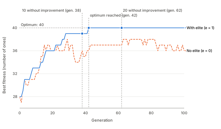
To find out, we programmed a genetic algorithm with the operators from the previous chapters and applied it to a simple problem: OneMax, which consists of finding a 40-bit string with as many ones as possible. Fitness is the number of ones, so the optimum is 40, and we know it in advance. The algorithm uses a population of 20 individuals, binary tournament selection, one-point crossover with Pc = 0.8, bit-flip mutation with pm = 1/40, and generational replacement, with no elite or with one elite individual. Both runs start from the same initial population.
figuras/08-elitismo-parada.py in the book repository.
Show the figure data
Best fitness in the population at selected generations:
| Generation | 0 | 5 | 10 | 15 | 20 | 25 | 30 | 35 | 38 | 42 | 50 | 62 | 80 | 100 |
|---|---|---|---|---|---|---|---|---|---|---|---|---|---|---|
| Without elite | 28 | 30 | 32 | 37 | 36 | 36 | 36 | 34 | 36 | 36 | 37 | 37 | 38 | 36 |
| With elite | 28 | 31 | 33 | 35 | 36 | 37 | 39 | 39 | 39 | 40 | 40 | 40 | 40 | 40 |
With an elite, the best fitness rises in steps and never falls: each improvement is kept until another one appears. Without an elite, it initially rises in a similar way, but, especially from generation 15 onward, it goes up and down: improvements are found and then lost again. In this run, the algorithm without an elite does not reach the optimum within 100 generations; with an elite, it reaches it at generation 42.
A single run is not enough to draw conclusions, because the result depends on chance (we saw this in exercise 5.6). So we repeated the experiment with 30 different seeds. Without an elite, 17 of the 30 runs reached the optimum within 100 generations; with an elite, all 30 did, and more than half did so in 33 generations or fewer.
Does it always help this much? No. OneMax has a single peak, and on problems like this elitism helps a great deal. De Jong found that elitism improved results on functions with a single optimum but worsened them on a function with many local optima: it improves local search at the expense of the global view (Goldberg, 1989, p. 115). If the elite dominates the population, its copies crowd out the others and diversity is lost sooner; the population may converge prematurely on a local optimum (Talbi, 2009, p. 221). That is why the elite is usually small, one or two individuals.
In figure 8.1, without an elite, the best fitness at generation 80 is 38 and at generation 100 it is 36. If the algorithm stopped at generation 100 and returned the best individual in the last population, what would its fitness be? What should the algorithm do so as not to lose the 38?
Show the solution
It would return an individual with fitness 36, even though it had found one with 38. Without an elite, the algorithm must store the best solution found so far separately and update it every generation; when it stops, it returns that solution, not the best in the last population. With an elite, the two coincide, because the best individual found is always in the population.8.6 When to Stop? BasicB
The cycle of selection, crossover, mutation, and replacement can be repeated indefinitely. When do we consider the search finished?
When it stops, the algorithm returns the best solution found, as we saw in exercise 8.5. The most common stopping criteria are of two kinds (Talbi, 2009, pp. 198–199):
- Fixed in advance. It is known from the start when the search will end: a maximum number of generations, a computing-time limit, or a maximum number of fitness-function evaluations. These criteria reflect limited resources. Evaluation may be the most expensive part: if each evaluation takes an hour, 10 000 evaluations take more than a year, about 50 generations with a population of 200 (Whitley, 1994, Section 1.1).
- Dependent on the search. It is not known in advance when they will be met:
- The optimum has been reached, or a good enough solution. This requires knowing the optimum or a bound on its value, which is uncommon.
- k generations have passed without improvement in the best solution found.
There are also criteria that look at the population’s diversity; we will see them in section 8.9.
In figure 8.1, the run with an elite shows what each criterion would do:
| Criterion | Stops at generation | Best fitness found |
|---|---|---|
| 10 generations without improvement | 38 | 39 |
| Optimum reached (40) | 42 | 40 |
| 20 generations without improvement | 62 | 40 |
| Maximum of 100 generations | 100 | 40 |
With 10 generations without improvement, the algorithm stops at generation 38, just before finding the optimum. With 20, it finds the optimum but then continues for 20 generations without gaining anything. With a maximum of 100 generations, the last 58 contribute nothing. Waiting too little can leave the search half-finished; waiting too long wastes resources. That is why criteria are often combined: for example, stop when the optimum is reached, if it is known, or after 20 generations without improvement, and in any case after 100 generations.
A genetic algorithm with an elite is maximizing a problem whose optimum is 50. This is the best fitness in its population at each generation:
| Generation | 0 | 1 | 2 | 3 | 4 | 5 | 6 | 7 | 8 | 9 | 10 |
|---|---|---|---|---|---|---|---|---|---|---|---|
| Best fitness | 31 | 35 | 35 | 42 | 42 | 42 | 47 | 47 | 47 | 47 | 50 |
At which generation does it stop under each criterion: (a) 3 generations without improvement; (b) 5 generations without improvement; (c) reaching the optimum; (d) a maximum of 8 generations? What fitness does it return in each case? If a criterion is not met before generation 10, assume the algorithm continues and no longer improves. (e) Combine (b) and (c): stop when the optimum is reached or after 5 generations without improvement, whichever comes first. (f) Now you do not know the optimum, and each generation takes one hour. Which two criteria would you combine, and why?
Show the solution
We count generations since the last improvement: there were improvements at generations 1, 3, 6, and 10.
- At generation 5, 2 generations have passed without improvement since generation 3; at generation 9, 3 have passed since generation 6. It stops at generation 9 and returns 47.
- Before generation 10, 5 consecutive generations without improvement never occur. At generation 10 the optimum is reached and cannot be improved, so it stops at generation 15 and returns 50, after five generations that contribute nothing.
- It stops at generation 10 and returns 50.
- It stops at generation 8 and returns 47.
- It stops at generation 10 and returns 50: the optimum arrives before the 5 generations without improvement.
- Without the optimum, (c) is useless. A reasonable option is (b) with a maximum number of generations that limits the time, such as (d): with this table it would stop at generation 8 with 47, after 8 hours. With (b) alone it would have reached 50, but after 15 hours. There is no single answer: it depends on how much going from 47 to 50 is worth compared with 7 more hours of computation, and in a real case we would not know that 50 arrives at generation 10.
Summary
- Replacement decides who forms the next generation. In generational replacement, the offspring replace all the parents; in steady-state replacement, only a few offspring come in at each step.
- With pure generational replacement, the best solution can be lost. Elitism passes the e best, unchanged, to the next generation; as a result, the best fitness never falls.
- Elitism speeds up the search, but it can reduce diversity and lead to premature convergence. That is why the elite is usually small.
- The algorithm stops when it reaches the optimum, if known, when it exhausts its resources, or when it has gone several generations without improvement. It returns the best solution found.
To continue along the basic path, go to “Parameters and Randomness”.
8.7 Steady-State Variants AdvancedA
If each offspring replaces a member of the population, does it matter much which one?
Between generational replacement and steady-state replacement with a single offspring there are intermediate positions: at each step, any number λ of individuals between 1 and μ can be replaced (Talbi, 2009, p. 221). De Jong (1975) called the fraction G of the population renewed in each generation the generation gap: G = 1 is generational replacement, and G < 1 is a population that overlaps with the previous one (Goldberg, 1989, p. 111; Mitchell, 1996/1998, Section 5.4). In De Jong’s model, the offspring took population slots chosen at random (Goldberg, 1989, p. 111).
selection-ga offers three rules for choosing whom each offspring replaces:
- Replace the worst, as in GENITOR. It is highly elitist: the best is never lost.
- Replace the oldest: the individual that has been in the population longest leaves, whether good or bad. Each individual lives for a fixed number of steps. The tool shows each parent’s age in the Age row; a newcomer starts at age 0, and everyone ages by one at each step.
- Replace a random one: replacement adds no pressure, and all the pressure comes from parent selection.
Choosing whom to replace is one decision; another is whether the offspring always enters or only when it is better than the individual it would replace. A widely used combination is to replace the worst only if the offspring is better (Lozano et al., 2008, p. 4422). In selection-ga this is the Replace the worst if better variant.
The choice changes selection pressure considerably. Goldberg and Deb showed that replacing the worst creates much greater pressure than replacing at random (Whitley, 1994, Section 8.1). Replacing the worst improves mean fitness quickly but can lead to premature convergence; that is why it is usually combined with large populations or with a rule that does not admit duplicate individuals (Eiben & Smith, 2015, pp. 88–89). Replacing a random individual has another drawback: De Jong and Sarma observed that its results varied more than those of a comparable generational algorithm, and Smith and Vavak explained this by showing that it loses the best much more often than replacing the oldest does. For this reason it is not recommended (Eiben & Smith, 2015, p. 88).
The name “steady state” can be misleading: these algorithms vary more than generational ones, which makes them more sensitive to sampling errors and genetic drift. In return, because GENITOR keeps the best points found, the search is more aggressive and is usually quite effective in practice (Whitley, 1994, Section 8.1). According to De Jong and Sarma, when steady-state replacement performs better than generational replacement, it is not because generations overlap but because of its greater selection pressure and the selection and replacement rules it uses (Lozano et al., 2008, pp. 4421–4422).
Data. The parents and the two offspring from example 8.4 (A–F: 12, 30, 5, 21, 9, and 17; a: 25; b: 14). The parents’ ages are:
| Parent | A | B | C | D | E | F |
|---|---|---|---|---|---|---|
| Fitness | 12 | 30 | 5 | 21 | 9 | 17 |
| Age | 2 | 5 | 3 | 1 | 2 | 3 |
Predict. What happens to B if the oldest is replaced? When ages are tied, the tool replaces the first one. With random replacement, can B be lost?
Open: replace the oldest Open: replace a random one
Show the result
| Variant | Next generation | Best fitness | Mean fitness |
|---|---|---|---|
| Replace the worst (example 8.4) | A B a D b F | 30 | 19.8 |
| Replace the oldest | A a b D E F | 25 | 16.3 |
| Replace a random one | a b C D E F | 25 | 15.2 |
Take the same parents, the Replace the worst variant, and two offspring, a (25) and b (3). Does b enter the population, even though it is worse than all the parents? Whom does it replace?
Show the solution
With Replace the worst, each offspring enters unconditionally. Offspring a replaces C (5), the worst. After that, the worst is E (9), and b replaces it even though b is worse: the next generation is A B a D b F, with mean 18. You can check this with the exercise link. With Replace the worst if better, b does not improve on E and is discarded: the next generation is A B a D E F, with mean 19 (link).- Change the Variant and click Random population several times. With which variant is the best lost most often?
- With Replace the oldest, follow the Age row step by step. Can a newly arrived offspring be replaced by the next one?
8.8 (μ + λ), (μ, λ), and Larger Elites AdvancedA
What if parents and offspring competed together to stay in the population?
Evolution strategies, created by Rechenberg and Schwefel in the sixties at the Technical University of Berlin, use two other replacement schemes. These schemes appeared in the seventies, when the strategies moved from a single parent and a single offspring to populations of μ parents and λ offspring (Eiben & Smith, 2015, p. 101; Whitley, 1994, Section 8):
- (μ + λ). The μ parents create λ offspring, and the μ best of the μ + λ individuals survive. A parent stays in the population until offspring better than it appear.
- (μ, λ). The offspring replace the parents, and selection takes place among the offspring alone: the μ best of the λ survive. This requires \lambda \geq \mu.
(μ + λ) is elitist: the best is never lost. (μ, λ) is not, and it resembles the generational replacement of the canonical genetic algorithm (Affenzeller et al., 2009, pp. 9–10). GENITOR also keeps the best solution by replacing the worst (Eiben & Smith, 2015, p. 89; Whitley, 1994, Section 8.1). But admitting any offspring, even one worse than the individual it replaces, is not exactly the same as (μ + λ): the mean can fall. In exercise 8.7, after a enters, the mean is 19, and when b, worse than E, enters, it falls to 18.
With a single offspring, Replace the worst if better is equivalent, in fitness, to keeping the μ best among the population and that offspring: it is (μ + 1). If several offspring are created, one must specify whether they are inserted one at a time under that condition or selected together from all the candidates.
Elitism with e individuals lies between the two schemes, although it matches neither. With e = 0 it is pure generational replacement. The larger e is, the more parents stay, but without competing with the offspring as in (μ + λ): the e best parents stay even if some discarded offspring is better than they are.
Data. The usual parents (A–F: 12, 30, 5, 21, 9, and 17) and nine offspring (λ = 9):
| Offspring | a | b | c | d | e | f | g | h | i |
|---|---|---|---|---|---|---|---|---|---|
| Fitness | 25 | 3 | 18 | 9 | 14 | 7 | 28 | 11 | 20 |
Predict. Who survives under (μ + λ)? And under (μ, λ)? How many parents remain in each case?
Show the result
| Scheme | Survivors, from best to worst | Parents | Best fitness | Mean fitness |
|---|---|---|---|---|
| (μ + λ) | B g a D i c (30, 28, 25, 21, 20, 18) | 2 | 30 | 23.7 |
| (μ, λ) | g a i c e h (28, 25, 20, 18, 14, 11) | 0 | 28 | 19.3 |
Why use a scheme that can lose the best? Because always keeping the best has the price we saw in section 8.5: the population loses diversity quickly and may converge prematurely (Talbi, 2009, p. 221). With (μ + λ), a very good individual can stay in the population indefinitely. With (μ, λ), no individual lasts more than one generation.
In evolution strategies, (μ, λ) is usually preferred, with many more offspring than parents: λ is typically 5 to 7 times μ. Because it discards all the parents, it can escape small local optima; if the problem changes over time, it does not cling to outdated solutions; and it does not hinder self-adaptation, in which the mutation parameters evolve together with each solution (Eiben & Smith, 2015, pp. 80, 89–90).
With parents A–F (12, 30, 5, 21, 9, and 17) and the six offspring from example 8.2 (25, 3, 18, 9, 14, and 7):
- Who survives under (μ, λ) with λ = μ = 6? Compare this with pure generational replacement.
- Who survives with elitism and e = 2?
Show the solution
- With λ = μ there is nothing to choose: all six offspring survive, as in pure generational replacement. The tool orders them from best to worst (a c e d f b), but they are the same individuals. The best fitness falls to 25.
- The elite consists of B (30) and D (21), which take the places of the two worst offspring, b (3) and f (7). The survivors are B D a c d e, with mean 19.5.
- In (μ + λ) selection, move the Number of offspring λ from 1 to 12. How many parents survive when there are few offspring? And when there are many?
- In (μ, λ) selection, set λ equal to μ and check that all the offspring survive. Then increase λ: what happens to the survivors’ mean fitness?
- In Generational with elitism, raise the Elite size e from 0 to 3 with the same population and watch how the proportion of parents and offspring changes.
8.9 Further Reading Further reading+
Replacing the most similar. De Jong sought a replacement scheme that would maintain diversity on functions with many optima, where elitism worsened results. He drew inspiration from nature: when similar individuals fill a niche, they compete more with one another. In his crowding model (De Jong, 1975, Section 4.7), with a generation gap G = 0.1, each offspring replaced the individual most similar to it among a few chosen at random; their number is the crowding factor, CF. With CF = 2 he obtained near-optimal results on a function with many local optima (Goldberg, 1989, p. 116). Other authors later developed the ideas of crowding and niching, which are important in optimizing functions with many optima (Goldberg, 1989, p. 116). One of them is Mahfoud’s deterministic crowding: parents are paired, each pair has two offspring, and each offspring competes with the parent most similar to it; the better of the two stays. The population spreads across several peaks, with subpopulations of similar size even when some peaks are better than others (Eiben & Smith, 2015, p. 94; Lozano et al., 2008, p. 4423).
Useful diversity. Lozano, Herrera, and Cano combine diversity with the pressure of replacing the worst. Among the individuals worse than the offspring, they look for the one that contributes least diversity, measured by its distance to its nearest neighbor. If the offspring contributes more diversity than that individual, it replaces it; if not, the offspring replaces the worst, provided it is better. In their experiments, this combination worked better than either rule alone and better than several crowding methods (Lozano et al., 2008, pp. 4424–4427).
An elite that also mutates. Keeping only the best is sometimes called the “golden cage model”. If mutation is applied to the elite to avoid premature convergence, the scheme is called weak elitism: the elite no longer passes intact (Affenzeller et al., 2009, p. 10).
Sometimes choosing the worst. If replacement always keeps the best, convergence is faster, but it may be premature. Sometimes it pays to keep bad individuals to avoid sampling errors (Talbi, 2009, p. 221). This is the same tension between selection pressure and diversity that we saw with truncation in chapter 5.
Noisy fitness. In some problems, an individual’s fitness is random: two evaluations of the same individual give different values, for example because they come from a simulation. Keeping the best from one generation to the next, as (μ + λ) does, makes it possible to re-evaluate them and estimate their fitness more and more reliably (Mitchell, 1996/1998, Section 5.4).
Stopping when the population stagnates. Stopping criteria specific to population-based algorithms look at the state of the population, above all its diversity: the run stops when diversity falls below a threshold (Talbi, 2009, p. 199). To use them, diversity must be measured, for example by the number of distinct individuals or by the mean distance between them.
Restarting instead of stopping. If the population has converged without finding a good enough solution, continuing to spend evaluations in the same region does not pay off. The search can be restarted with a new, highly diverse population while keeping the best solution found (García-Martínez et al., 2025, p. 641). Eshelman’s CHC algorithm restarts when diversity falls below a threshold: it creates the new population from the best individual, randomly changing 35% of its bits, and if several consecutive restarts bring no improvement, it creates the population entirely at random. Micro-genetic algorithms work with very small populations, of about five individuals, which converge quickly; when they converge, they keep the best and replace the others with random individuals (García-Martínez et al., 2025, pp. 641–642).
No duplicate individuals. Another simple way to preserve diversity is not to admit copies: for example, discarding an offspring that is already in the population. Early empirical studies already showed that removing duplicates can improve results considerably (García-Martínez et al., 2025, p. 643).
Replacement as a parameter. The type of replacement can also be tuned. Grefenstette (1986, pp. 124, 126) used a genetic algorithm to search for the parameters of another, including the generation gap and whether elitism was used; the best setting for one of his performance measures used G = 1 and elitism (Mitchell, 1996/1998, Section 5.6). But such recommendations depend on the test functions with which they were obtained.