3 Representing Solutions
Tools: representation-ga, available through the portal.
After completing the basic path through this chapter, you will be able to:
- distinguish genotype, phenotype, and decoding, and decode a given chromosome;
- read and write binary numbers and calculate the precision provided by a given number of bits;
- write an assignment as an integer vector and a tour as a permutation, and recognize a chromosome that is not a permutation;
- explain why a real-valued vector needs no decoding and identify the problem it still faces;
- distinguish a valid chromosome from a feasible solution, and check whether a selection of items fits in a knapsack;
- choose a representation according to the type of decision in the problem.
3.1 Genotype and Phenotype BasicB
Problems describe machines, cities, or real numbers, but genetic algorithms manipulate chromosomes. How are the two connected?
A chromosome is a string of genes, each taking a value, its allele (Mitchell, 1996/1998, Section 1.3). The string is the genotype, what crossover and mutation manipulate. Its corresponding solution is the phenotype, what makes sense in the problem and is evaluated (Talbi, 2009, p. 34, note 25). Converting one to the other is decoding. The representation, or encoding, defines the whole arrangement: which chromosomes exist and which solution each describes (Talbi, 2009, p. 40).
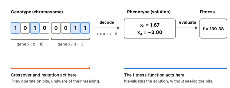
figuras/03-representacion.py in the book repository.
The diagram captures an idea used throughout this chapter: crossover and mutation do not know what the bits mean, and the fitness function does not see the bits. Everything between them—the representation—determines which solutions are reachable, how changing a gene changes the solution, and whether operators can produce chromosomes describing no solution. Choosing a representation therefore requires thinking about evaluation and operators together (Talbi, 2009, p. 35).
Consider a complete decoding example. We seek the lowest point of Himmelblau’s function,
f(x_1, x_2) = (x_1^2 + x_2 - 11)^2 + (x_1 + x_2^2 - 7)^2,
inside the square [-5, 5]^2. Here f is the objective function being minimized: lower is better. The tool and figure 3.1 call this value “Fitness”; other examples maximize it. Always check which direction is better. Cost is transformed into an increasing fitness only when a mechanism, such as roulette-wheel selection, requires it (section 4.6).
Each variable is written using k = 4 bits. These are read as an integer z from 0 to 15, then spaced equally between −5 and 5. Section 3.2 develops the formula.
Figure 3.2 shows the function. It has four minima, all with f = 0, each in its own valley. Between them, near (-0.27, -0.92), lies a local maximum with f \approx 181.6. The function rises toward the corners, reaching 890 at (5, 5).
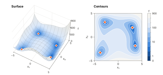
figuras/03-himmelblau.py in the book repository.
Data. Chromosome 1 0 1 0 0 0 1 1, with k = 4. The first four bits encode x_1 and the next four encode x_2. Consecutive representable values are separated by \Delta = 10/15 \approx 0.6667, and the formula is x = -5 + z\,\Delta.
Predict. What are z_1 and z_2? Which point does the chromosome represent? What is f there?
Show the result
The first group, 1010, gives 8 + 2 = 10; the second, 0011, gives 2 + 1 = 3. Thus,
x_1 = -5 + 10 \times 0.6667 \approx 1.6667, \qquad x_2 = -5 + 3 \times 0.6667 = -3.
The chromosome represents (1.6667, -3), where f \approx 139.38. The function’s minimum is 0, so this individual is far from it. Between two individuals, the one with lower f is better.Show the tool here (decode the chromosome)
Mutating just one bit, for example the first, gives 0 0 1 0 0 0 1 1: z_1 changes from 10 to 2 and x_1 from 1.6667 to −3.6667. One bit moves the point by 8\,\Delta \approx 5.33, more than half the box’s side length. This is a consequence of the representation, not a malfunction; section 3.8 returns to it.
Using the same representation (Himmelblau, [-5, 5]^2, k = 4), decode 0 0 0 0 1 1 1 1 and calculate f. Can any chromosome represent (0, 0) exactly? What about (1, −1)? If so, write it.
Show the solution
The first four bits give z_1 = 0, so x_1 = -5; the last four give z_2 = 15, so x_2 = -5 + 15 \times 10/15 = 5. The point is (-5, 5), a corner of the box, and f = (25 + 5 - 11)^2 + (-5 + 25 - 7)^2 = 19^2 + 13^2 = 530.
Representing x = 0 would require z = 5/\Delta = 7.5, which is not an integer. No chromosome of this type represents (0, 0); the nearest values use z = 7 or z = 8, giving x = \mp 0.3333.
Encoding reverses the process: point to z, then z to bits. For x_1 = 1, we need z_1 = 6/\Delta = 9; for x_2 = -1, z_2 = 4/\Delta = 6. Both are integers, so (1, −1) lies on the grid: 9 = 1001 and 6 = 0110, giving chromosome 1 0 0 1 0 1 1 0.- Use Next to move through Problem, Formalisation, Encoding, Exploration, and Validity. At which stage does the chromosome appear, and at which does the point appear?
- Click a chromosome bit and watch the point move on the map. Which bits move it a long way, and which move it only slightly?
- Click Random chromosome several times and record each point’s f value.
3.2 Binary: Integers and Real Numbers BasicB
If every gene is a bit, how do bits represent a number?
Binary representation uses an alphabet of two symbols. It naturally describes yes-or-no decisions, such as which items enter a knapsack (Talbi, 2009, p. 36), and can also represent numbers (Goldberg, 1989, pp. 80–82; Mitchell, 1996/1998, Section 5.2). An unsigned integer is read in base 2: for k bits b_1 b_2 \dots b_k, with b_1 most significant,
z = \sum_{j=1}^{k} b_j\, 2^{\,k-j}, \qquad z \in \{0, 1, \dots, 2^k - 1\}.
To represent a real number in [a, b], map this integer linearly into the interval so that 00…0 gives endpoint a and 11…1 gives endpoint b (Goldberg, 1989, p. 82):
x = a + z\,\Delta, \qquad \Delta = \frac{b - a}{2^k - 1}.
The step Δ is the precision of the representation: the distance between two consecutive representable values. For several variables, give each its own k bits and concatenate the groups, as in figure 3.1 (Goldberg, 1989, pp. 82–83). With n variables and k bits per variable, the chromosome has n \times k bits and the search space contains 2^{nk} chromosomes. Each variable can take only 2^k values.
A notation detail: we divide by 2^k - 1 because the largest representable integer is 2^k - 1, making both a and b representable. Dividing by 2^k would leave endpoint b unreachable.
A parameter ranges from 2.5 to 20.5 and is written with 8 bits. What value does chromosome 1 0 1 0 0 0 1 1 represent? How many distinct values are available, and how far apart are consecutive ones?
Show the solution
Read as one integer, the 8 bits give z = 128 + 32 + 2 + 1 = 163. With k = 8, there are 2^8 = 256 values and \Delta = (20.5 - 2.5)/255 \approx 0.0706. The represented value is x = 2.5 + 163 \times 18/255 \approx 14.006.
Compare this with example 3.1: the same bits now encode one 8-bit variable instead of two 4-bit variables. Chromosomes have no meaning by themselves; meaning comes from the representation.3.3 Binary: How Many Bits Are Needed? BasicB
With k bits, each variable has only 2^k possible values. What is lost along the way?
Every value between consecutive representable values is lost. The desired solution, such as a function’s minimum, may not be representable. To show how this changes with bit count, figure 3.3 plots Himmelblau’s representable points for k = 3, 4, and 5.
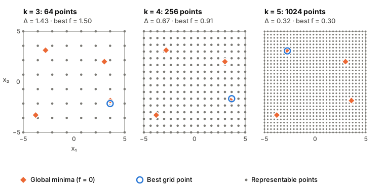
figuras/03-representacion.py in the book repository.
Show the figure data
| Bits per variable k | Points | Δ | Best representable point | f at that point |
|---|---|---|---|---|
| 3 | 64 | 1.4286 | (3.5714, −2.1429) | 1.504 |
| 4 | 256 | 0.6667 | (3.6667, −1.6667) | 0.9136 |
| 5 | 1 024 | 0.3226 | (−2.7419, 3.0645) | 0.2971 |
Adding one bit per variable roughly halves point spacing. But with two variables, it also multiplies the chromosome count by four: 2^{2k}. Greater precision comes at the cost of a larger search space.
Data. Himmelblau’s function on [-5, 5]^2 with k = 3, 4, and 5 bits per variable. Each chromosome merely opens the tool at a sample point; the questions do not depend on that chromosome.
Predict. How many chromosomes are there in each case, and what is Δ? Does the best representable point reach 0? Does it always lie in the same valley?
Open: k = 3 Open: k = 4 Open: k = 5
Show the result
There are 2^6 = 64, 2^8 = 256, and 2^{10} = 1\,024 chromosomes, with \Delta = 10/7 \approx 1.4286, 10/15 \approx 0.6667, and 10/31 \approx 0.3226. No grid contains an exact minimum, so the best representable values are not 0: they are 1.504, 0.9136, and 0.2971. More bits improve the result here, but not always in the same valley: for k = 3 and k = 4, the best point lies near the lower-right minimum; for k = 5, near the upper-left one. The finer grid is not a refinement containing the previous grid, because their points do not coincide.With k = 10 bits per variable, precision is already about one hundredth (\Delta \approx 0.0098), the best representable value is 0.0005, and the chromosome’s 20 bits allow more than a million distinct chromosomes. Choosing k balances precision against search-space size. More bits do not even guarantee a better representable point: at k = 7 the best value is 0.00026, but at k = 8 it is 0.0035, because the grids differ.
We want consecutive values of a variable in [-5, 5] to be at most 0.01 apart. How many bits does each variable need? How many bits does the Himmelblau chromosome then contain?
Show the solution
We need 10/(2^k - 1) \le 0.01, or 2^k - 1 \ge 1\,000. With k = 9, 2^9 - 1 = 511 and \Delta \approx 0.0196, which is insufficient. With k = 10, 2^{10} - 1 = 1\,023 and \Delta \approx 0.0098, which is sufficient. Each variable needs 10 bits, making a chromosome of 2 \times 10 = 20.- Advance to Validity, change Bits per variable (k) from 2 to 12, and inspect Δ and “Best on the grid.” From which k onward is that value below 0.1?
- At Validity, check that every string lies inside the box: binary encoding cannot leave it.
- Switch to Rastrigin, whose optimum is at the origin. Does any k give a grid containing (0, 0)? Reason it out, then check several values of k. Exercise 3.1 may help.
3.4 Integer: One Number per Decision BasicB
A workshop has several machines, and each task runs on exactly one. How can a schedule be written as a chromosome?
In integer representation, each gene is an integer within a range, and values may repeat. It suits problems where each variable chooses among options, such as assignment (Talbi, 2009, p. 36). Here gene i identifies the machine processing task i. With n tasks and m machines, the chromosome has n genes, each from 1 to m.
Our example has 5 tasks and 3 machines. Each machine takes a different time for each task:
| Task | Machine 1 | Machine 2 | Machine 3 |
|---|---|---|---|
| 1 | 4 | 6 | 3 |
| 2 | 5 | 2 | 7 |
| 3 | 3 | 3 | 5 |
| 4 | 6 | 4 | 2 |
| 5 | 2 | 5 | 6 |
Machines work simultaneously. A machine’s load is the sum of its assigned task times, and the makespan, C_{\max}, is the largest load: when the final machine finishes. We want to minimize it. The constraint requires each task to run on one machine, and only one.
This representation satisfies the constraint automatically: each gene holds one number, so every task has exactly one machine. The gene domain is said to absorb the constraint. All 3^5 = 243 possible chromosomes are valid assignments.
Data. The table’s processing times and chromosome 2 1 3 2 1: task 1 goes to machine 2, task 2 to machine 1, task 3 to machine 3, task 4 to machine 2, and task 5 to machine 1.
Predict. What is each machine’s load? What is the makespan?
Show the result
| Machine | Tasks | Load |
|---|---|---|
| 1 | 2 and 5 | 5 + 2 = 7 |
| 2 | 1 and 4 | 6 + 4 = 10 |
| 3 | 3 | 5 |
Show the tool here (assignment 2 1 3 2 1)
The genes are integers, but they are not quantities here: machine 3 is no “closer” to machine 2 than to machine 1. They are labels, or nominal values. In other problems, integers do represent ordered quantities, such as batch units or workers on a shift; nearby values then often give similar solutions (Eiben & Smith, 2015, Section 4.3). This distinction determines which operators make sense, as section 7.3 in the mutation chapter explains.
Start with chromosome 2 1 3 2 1 from example 3.4. (a) Move task 4 to machine 3. What is the new chromosome and makespan? (b) Instead, move task 1 to machine 3. What happens now? (c) Which change is better?
Show the solution
The chromosome is 2 1 3 3 1. Task 4 leaves machine 2 (load 10 - 4 = 6) for machine 3, where it takes 2: load 5 + 2 = 7. The loads are 7, 6, and 7; makespan is 7.
The chromosome is 3 1 3 2 1. Task 1 leaves machine 2 (load 10 - 6 = 4) for machine 3, where it takes 3: load 5 + 3 = 8. The loads are 7, 4, and 8; makespan is 8.
The first change is better, with makespan 7. Both results remain valid assignments: this integer representation has no invalid chromosomes.
- Click a chromosome gene to move its task to the next machine and watch loads and makespan change.
- Try to reach the optimal makespan, shown by the dashed line, using only gene changes. How many changes do you need?
- Click Random instance to try other processing times.
3.5 Permutations: An Ordering BasicB
A traveler must visit each of n cities exactly once. Would an integer vector like the assignment encoding work?
An integer vector allows repeated values, but a tour cannot repeat cities. Permutation representation describes an order: each gene is a city, and each city appears exactly once. Gene j gives the city visited in position j; the traveler returns from the last city to the first (Talbi, 2009, p. 36). This representation suits sequencing, scheduling, and routing problems.
Here, the constraint that each city be visited once is enforced not by each gene’s domain but by the structure of the whole chromosome. A valid chromosome meets that structure: it is a permutation. Permutations therefore need operators that preserve it, such as those in chapters 6 and 7.
There is another feature. With n cities, there are n! permutations, but the same tour has many descriptions: it can start at any of its n cities and run in either direction. Thus, each tour has 2n chromosomes, leaving only (n-1)!/2 distinct tours. When several chromosomes represent the same solution, this is called redundancy.
Data. A problem with n = 6 cities (seed 3) and chromosome 1 3 5 2 6 4. The tour leaves city 1, visits 3, 5, 2, 6, and 4, then returns to 1.
Predict. How many permutations and distinct tours are there? How many chromosomes describe this tour? How long is tour 4 6 2 5 3 1?
Show the result
There are 6! = 720 permutations and 5!/2 = 60 distinct tours. Each tour has 2n = 12 chromosomes: the 6 rotations, such as 3 5 2 6 4 1, and the 6 rotations of the reverse order, such as 4 6 2 5 3 1. All describe the same solution with length 327.4. Tour 4 6 2 5 3 1 follows the route backward and has the same length.
That 327.4 is far from the optimum, 239.6, given by tour 1 3 5 6 4 2. Swapping two cities, for example 1 and 2, gives 2 3 5 1 6 4, a different tour of length 327.7.Show the tool here (tour 1 3 5 2 6 4)
(a) With 6 cities, is chromosome 1 3 5 3 6 4 valid? If not, what is wrong? (b) A simple repair scans the chromosome and replaces each repeated city by the smallest missing city. What chromosome results? (c) With n = 10 cities, how many permutations and distinct tours exist?
Show the solution
It is invalid: city 3 appears twice, and city 2 is missing. It describes no tour.
City 3 appears a second time at position 4; the smallest missing city is 2. The result is 1 3 5 2 6 4, the tour in example 3.5.
There are 10! = 3\,628\,800 permutations and 9!/2 = 181\,440 distinct tours. With just 10 cities, the chromosome space already contains over three and a half million elements.
- Click two genes to swap them and check that the result remains a permutation. How much does tour length change?
- Click Invalid chromosome to see a repeated city and follow the Repair step.
- Find the current chromosome in Equivalent chromosomes and check that all twelve have the same length.
3.6 Real-Valued: The Chromosome Is the Point BasicB
If a problem already uses real numbers, must we convert them to bits?
No. In real-valued representation, the chromosome is a vector of real numbers with one gene per variable. This is the natural encoding for continuous optimization (Talbi, 2009, p. 37). Genotype and phenotype coincide: no decoding is needed, and a Himmelblau chromosome is the point (x_1, x_2) itself. Precision no longer depends on a bit count but on the machine (the tool stores genes to hundredths).
This has advantages. There is no k to choose, intermediate values are not lost to a binary grid, and operators act directly on problem values, as do arithmetic crossover and Gaussian mutation in chapters 6 and 7. It is also the most natural representation in many applications. There are no rigorous rules saying which of binary and real-valued encoding works better, however; that depends on the problem and algorithm details (Mitchell, 1996/1998, Section 5.2).
Data. Himmelblau’s function on [-5, 5]^2 and real-valued chromosome (3, 2).
Predict. What is f at this point? Can binary encoding with k = 4 bits per variable represent it?
Show the result
f(3, 2) = (9 + 2 - 11)^2 + (3 + 4 - 7)^2 = 0: this is one of the four global minima. A real-valued vector represents it exactly.
With k = 4 bits, x_1 = 3 is representable (z_1 = 12), but x_2 = 2 requires z_2 = 7/\Delta = 10.5, not an integer. More bits do not solve this: x_2 = 2 requires z = 7\,(2^k - 1)/10, and 2^k - 1 is always odd, so this quantity is never an integer. No minimum lay on the grids in example 3.3.Show the tool here (point (3, 2))
A real-valued vector faces a problem binary encoding did not: a gene can take any real value, including one outside the permitted interval. Section 3.11 explains how to handle it.
Which representation would you choose for each problem, and what would a gene mean? (a) Decide which products from a catalog of 20 to include in an order. (b) Divide 12 deliveries among 4 drivers, each delivery assigned to exactly one. (c) Choose the order of 8 jobs on one machine. (d) Adjust three continuous model coefficients.
Show the solution
(a) A 20-gene bit vector: gene i is 1 if product i enters the order (a yes-or-no decision). (b) A 12-gene integer vector with values 1 to 4: gene i gives delivery i’s driver (an unordered category). (c) An 8-gene permutation: gene j is the job processed at position j. (d) A 3-gene real-valued vector: one coefficient per gene. This is natural, although binary encoding is possible with precision determined by its bit count.3.7 Valid Chromosomes and Feasible Solutions BasicB
Does every bit string describe something that can actually be carried out?
Two concepts must be distinguished. A chromosome is valid when it has the structure required by its representation: each city once in a permutation, or one in-range value per gene in an integer vector. The solution it describes is feasible when it meets the problem’s constraints (Talbi, 2009, p. 48). In the binary, integer, and permutation examples above, these coincide; real-valued vectors can leave the box (section 3.11). In the knapsack problem, the distinction arises even with bits.
The 0/1 knapsack problem has n items, each with weight w_i and value v_i, and capacity W. Choose items to maximize total value without exceeding capacity. It is a classic, difficult combinatorial optimization problem: for many items, no known method always finds the best selection in reasonable time (section 3.13). The natural representation is binary, one bit per item: gene i is 1 if item i is included (Talbi, 2009, p. 36). Every n-bit string is a valid chromosome describing a selection, but that selection is feasible only if \sum_i w_i x_i \le W.
We use 6 items and capacity W = 10:
| Item | 1 | 2 | 3 | 4 | 5 | 6 |
|---|---|---|---|---|---|---|
| Weight w_i | 3 | 5 | 2 | 4 | 6 | 1 |
| Value v_i | 4 | 6 | 3 | 5 | 7 | 2 |
Data. The table’s problem (W = 10) and chromosomes 1 0 0 1 0 1, 1 1 0 1 1 0, and 1 0 1 1 0 1.
Predict. What are each selection’s weight and value? Which are feasible? Which feasible selection is best?
Open: 100101 Open: 110110 Open: 101101
Show the result
| Chromosome | Included items | Weight | Value | Feasible? |
|---|---|---|---|---|
| 1 0 0 1 0 1 | 1, 4, 6 | 8 | 11 | Yes |
| 1 1 0 1 1 0 | 1, 2, 4, 5 | 18 | 22 | No: exceeds capacity by 8 |
| 1 0 1 1 0 1 | 1, 3, 4, 6 | 10 | 14 | Yes, weight equals W |
Show the tool here (chromosome 1 1 0 1 1 0)
Chromosome 1 1 0 1 1 0 has value 22, above the optimum 14, but does not fit. Evaluating value alone would make the algorithm think it was best. This is common: 28 of the 32 infeasible chromosomes exceed the optimum’s value, because including more items generally increases value. Infeasible chromosomes are therefore a real issue. We must reject them, repair them, use a decoder producing only feasible solutions, or penalize them—keep them in the population with worse fitness. Advanced section 3.10 compares these strategies; section 4.7 covers the most common, penalization.
When representation absorbs constraints, as the assignment integer vector does, this issue disappears. Choosing a representation partly determines how many constraints are handled by writing the chromosome and how many remain for later.
For the problem in example 3.7, are 0 1 1 0 0 1 and 0 1 1 0 1 1 feasible? What are their values? Is a 7-bit chromosome valid?
Show the solution
Chromosome 0 1 1 0 0 1 includes items 2, 3, and 6: weight 5 + 2 + 1 = 8 \le 10 and value 6 + 3 + 2 = 11. It is feasible.
Chromosome 0 1 1 0 1 1 includes items 2, 3, 5, and 6: weight 5 + 2 + 6 + 1 = 14 > 10 and value 6 + 3 + 7 + 2 = 18. It is infeasible, exceeding capacity by 4.
A 7-bit chromosome is invalid: the problem has 6 items and requires one gene per item. This is a structural error, not a constraint violation.- Click genes and watch which items enter the knapsack and when excess capacity appears.
- At Formalisation, read how many chromosomes exist and how many are feasible.
- Click Random instance several times and compare feasible proportions. What do you think determines them?
Summary
- Representation defines how a solution is written. Genotype (chromosome) is manipulated by crossover and mutation; phenotype (solution) is evaluated; decoding connects them.
- Each decision type suggests a representation: bits for yes-or-no choices and interval-valued numbers, integers for choosing among options, permutations for ordering, and real values for continuous variables.
- Binary precision for a real number is \Delta = (b - a)/(2^k - 1): each extra bit refines the grid but enlarges the search space.
- A valid chromosome meets the representation’s structural rules; a feasible solution meets problem constraints. These are different concepts. Some representations absorb constraints; others require additional handling of violations.
To continue along the basic path, go to “Initialization and Evaluation”.
3.8 Binary: Hamming Cliffs and Gray Code AdvancedA
Mutating one bit ought to change the point only slightly. Does binary representation of real values do this?
A good representation should have locality: similar solutions should have similar chromosomes, and vice versa, with similarity measured through the operators used (Talbi, 2009, p. 43). Standard binary encoding does not meet this requirement for bit-changing operators. Consider integers 15 and 16. They are neighbors, but their 5-bit strings are 0 1 1 1 1 and 1 0 0 0 0: moving between them requires changing all five bits (Talbi, 2009, p. 43). This jump between neighboring solutions with distant chromosomes is a Hamming cliff. Conversely, as example 3.1 showed, changing a variable’s most significant bit moves the point by slightly more than half the box.
Reflected Gray code makes consecutive integers differ in exactly one bit (Mitchell, 1996/1998, Section 5.2). To convert standard binary b_1 b_2 \dots b_k to Gray, copy the first bit; each following bit is the exclusive OR (\oplus) of consecutive binary bits:
g_1 = b_1, \qquad g_j = b_{j-1} \oplus b_j \quad (j = 2, \dots, k).
\oplus gives 1 for different bits and 0 for identical bits. Decode by reversing the process: b_1 = g_1 and b_j = b_{j-1} \oplus g_j. Read b as an integer, then apply the formula in section 3.2.
| Integer z | 5 | 6 | 7 | 8 |
|---|---|---|---|---|
| Standard binary | 0101 | 0110 | 0111 | 1000 |
| Gray | 0111 | 0101 | 0100 | 1100 |
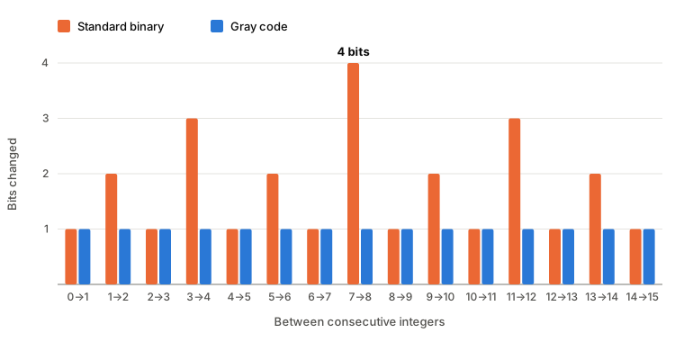
figuras/03-representacion.py in the book repository.
Show the figure data
Bits changed from z to z + 1, with k = 4:
| Transition | 0→1 | 1→2 | 2→3 | 3→4 | 4→5 | 5→6 | 6→7 | 7→8 | 8→9 | 9→10 | 10→11 | 11→12 | 12→13 | 13→14 | 14→15 |
|---|---|---|---|---|---|---|---|---|---|---|---|---|---|---|---|
| Standard | 1 | 2 | 1 | 3 | 1 | 2 | 1 | 4 | 1 | 2 | 1 | 3 | 1 | 2 | 1 |
| Gray | 1 | 1 | 1 | 1 | 1 | 1 | 1 | 1 | 1 | 1 | 1 | 1 | 1 | 1 | 1 |
Data. Himmelblau’s function with k = 4 and point (-0.3333, -0.3333), corresponding to z_1 = z_2 = 7. Standard binary encodes it as 0 1 1 1 0 1 1 1; Gray uses 0 1 0 0 0 1 0 0. Its grid neighbor along x_1 has z_1 = 8.
Predict. How many bits change in each code when moving from z_1 = 7 to z_1 = 8?
Open: standard binary Open: Gray code
Show the result
In standard binary, 0 1 1 1 becomes 1 0 0 0: 4 bits change. In Gray, 0 1 0 0 becomes 1 1 0 0: only 1 bit, the first, changes. Both chromosomes represent the same point, with f \approx 178.1.
Gray does not solve everything: of eight chromosomes one bit away, only four (50%) are grid neighbors (standard binary has two, 25%); the others jump farther. For example, changing the second bit in 0 1 0 0 gives 0 0 0 0, or z = 0, at the box’s edge.Show the tool here (Gray code)
Gray guarantees that a grid neighbor is one bit away, not that every one-bit change reaches a grid neighbor. Over 1 000 random points with k = 4, the tool finds that reaching a grid neighbor requires, in the worst case, an average of 2.9 gene changes in standard binary but always 1 in Gray (this differs from the average 1.73 bits changed between z and z + 1). Meanwhile, the proportion of one-bit neighbors that are grid neighbors rises from 25% to 48%, not to 100%. Gray removes Hamming cliffs between consecutive values but does not make every one-bit change local. Talbi identifies poor handling of dynamic ranges as its main drawback (Talbi, 2009, p. 43). Mitchell lists it among extensions of binary encoding (Mitchell, 1996/1998, Section 5.2).
(a) Write integer z = 5 in 4-bit Gray code. (b) What integer does Gray code 1 1 0 0 represent? (c) Write 15 and 16 in 5-bit standard binary and Gray, and count changed bits in each.
Show the solution
Binary 5 is 0101. Copy the first bit (0); the second is 0 \oplus 1 = 1; the third, 1 \oplus 0 = 1; the fourth, 0 \oplus 1 = 1. Gray code is 0 1 1 1.
Copy the first bit (1); next comes 1 \oplus 1 = 0, then 0 \oplus 0 = 0, and finally 0 \oplus 0 = 0. The binary string is 1000, or 8.
Standard binary uses 01111 for 15 and 10000 for 16: all 5 bits change. Gray uses 01000 for 15 and 11000 for 16: 1 bit changes.
- In the Locality table, compare Genes to the grid neighbour and Grid neighbours for standard binary and Gray. Bold values refer to this point; bracketed values average 1 000 random points.
- Increase Bits per variable (k) from 4 to 8. How does the average number of gene changes to a grid neighbor change in standard binary? What about Gray?
- Click Random point several times, looking for points where standard binary needs 1 bit change and others where it needs many.
3.9 Binary Matrix: When the Constraint Is Not Absorbed AdvancedA
The same assignment problem can use bits. What changes if each task–machine pair has a bit?
In a binary matrix, chromosome bit y_{ij} corresponds to task i and machine j, with y_{ij} = 1 when task i runs on machine j. For 5 tasks and 3 machines, there are 15 bits. Binary operators apply, but the one-machine-per-task constraint is no longer absorbed: a task can have no 1 (not processed) or several (processed on several machines). It must be checked, as in the knapsack.
This resembles section 3.7, but more strongly. Of 2^{15} = 32\,768 chromosomes, only 3^5 = 243 are feasible assignments: 0.74%. The rest describe no schedule.
Data. Processing times from example 3.4, and the binary matrix grouped into three bits per task: 0 0 0 | 1 1 0 | 0 0 1 | 0 1 0 | 1 0 0. Each group lists that task’s bits for machines 1, 2, and 3. Repair processes tasks in order: with no 1, assign the fastest machine; with several, keep the fastest among those selected. Break equal-time ties in favor of the lower machine number.
Predict. Is it feasible? Which tasks violate the constraint? What assignment results from repair, and what is its makespan?
Open: infeasible matrix and repair
Show the result
It is infeasible. Task 1 has no machine (000), and task 2 has two (110); the other three satisfy the constraint. Total violation v sums each task’s deviation from exactly one 1: v = |0 - 1| + |2 - 1| = 2.
Repair assigns task 1 to its fastest machine, 3 (time 3), and leaves task 2 on machine 2 (time 2 rather than 5 on machine 1). The assignment is 3 2 3 2 1, with loads 2, 6, and 8 and makespan 8. The optimum is 5.
This assignment is not represented by only one matrix: of 32 768 matrices, 250 repair to 3 2 3 2 1. Only one is feasible before repair.Show the tool here (matrix and repair)
The “Compare encodings” page contrasts both representations using the same problem and assignment 2 1 3 2 1 from example 3.4:
| Integer vector | Binary matrix | |
|---|---|---|
| Chromosome | 5 integers | 15 bits |
| Search space | 3^5 = 243 | 2^{15} = 32\,768 |
| Feasible chromosomes | 100% | 0.74% |
| Chromosomes giving the same assignment | 1 | 20 (mean over all assignments: 134.8) |
| One-gene neighbors | 10 | 15 |
| Neighbors that are assignments | 100% | 0% |
| Neighbors repeating the assignment after repair | 0% | 33% |
With the vector, any one-gene change gives another assignment. With the matrix, changing one bit never leaves a feasible assignment; one third of repairs return the same assignment, so the algorithm makes no move. Every matrix operator therefore needs a way to handle infeasible chromosomes. Section 3.10 lists the strategies.
Using the processing times from example 3.4, repair 1 1 1 | 0 0 0 | 0 1 0 | 0 0 1 | 0 0 0 with the rule from example 3.9. What assignment results?
Show the solution
Task 1 has three 1s; keep its fastest machine, 3 (time 3). Task 2 has none; assign its fastest machine, 2 (time 2). Tasks 3 (machine 2) and 4 (machine 3) already satisfy the constraint. Task 5 has none; assign its fastest machine, 1 (time 2). The assignment is 3 2 2 3 1.
This is one of the problem’s two optimal assignments. Loads are 2, 5, and 5: machine 1 processes task 5 (time 2), machine 2 processes tasks 2 and 3 (2 + 3 = 5), and machine 3 processes tasks 1 and 4 (3 + 2 = 5). Makespan is 5.- Check the search-space table against this section’s sizes, feasible percentages, and redundancy.
- Change Tasks and Machines and watch chromosome counts change. How many more become infeasible as the numbers of tasks and machines increase? (Random instance only draws new times at the same size.)
- Open each encoding’s name to view its page with the same instance and assignment.
3.10 Handling Infeasible Chromosomes AdvancedA
What should we do with a chromosome representing a solution that violates constraints?
Classic reviews group constraint-handling strategies somewhat differently (Coello Coello, 2002). Michalewicz and Schoenauer, for example, use four categories and include repair within methods distinguishing feasible from infeasible solutions (Michalewicz & Schoenauer, 1996, Section 3). We follow Talbi’s five categories (Talbi, 2009, p. 48), applying them to the overweight knapsack chromosome 1 1 0 1 1 0 from section 3.7.
- Reject. Discard infeasible chromosomes, the death penalty approach (Coello Coello, 2002, Section 2.7; Talbi, 2009, p. 49). This is reasonable only when they are rare, and loses the information they provide (Talbi, 2009, p. 49), which Richardson et al. (1989) already advised against simply discarding. Half the example knapsack chromosomes are infeasible; the binary matrix in section 3.9 has 99% infeasible chromosomes.
- Penalize. Accept the chromosome but reduce fitness according to its constraint violation (Talbi, 2009, pp. 49–50). This is the most common strategy (Coello Coello, 2002, Section 2; Talbi, 2009, p. 49). For the knapsack, let excess weight be e = \max(0, \text{weight} - W). A linear penalty gives fitness = value - \lambda\, e; a quadratic penalty gives value - (\lambda\, e)^2. If λ is too small, the algorithm ends with infeasible solutions; if too large, it remains with feasible but suboptimal solutions (Talbi, 2009, p. 50). Section 4.7 covers λ and penalty variants.
- Repair. A procedure, usually a greedy heuristic, turns an infeasible chromosome into a feasible one (Coello Coello, 2002, Section 4; Talbi, 2009, pp. 52–53). Apply it only to infeasible chromosomes; leave feasible ones untouched. For the knapsack, remove items until the selection fits. Greedy repair removes the worst value-to-weight ratio first; random repair removes any item. Michalewicz & Arabas (1994, p. 138) compared both. Chu & Beasley (1998, p. 74) used two phases: after removals, insert any items that still fit, in descending ratio order. Repair procedures are problem-specific (Talbi, 2009, p. 53).
- Decode. The chromosome is not the solution but instructions used by a decoder that always constructs a feasible solution (Coello Coello, 2002, Section 3.6; Talbi, 2009, p. 53). For the knapsack, scan genes in order; each 1 means “try to include this item,” adding it only if it fits.
- Preserve. Design representation and operators to produce only feasible solutions (Coello Coello, 2002, Section 3; Talbi, 2009, p. 53). Permutation operators in chapters 6 and 7 do this. The strategy is tailored to the problem.
Which works best? It depends. Michalewicz & Arabas (1994, pp. 140–141) compared penalties, repairs, and decoders for the knapsack. At small capacity, when few selections fit, penalties failed to reach feasible solutions and greedy repair performed best; at larger capacity, the gentlest, logarithmic penalty performed best.
Data. The knapsack from section 3.7 (W = 10) and infeasible chromosome 1 1 0 1 1 0, weight 18 and value 22. Both penalties use λ = 2. Random repair draws 0.62, 0.00, and 0.52; each chooses which of the q remaining items to remove: index \lfloor r\,q \rfloor, counting from 0 in gene order.
Predict. What fitness does each penalty give? Which items does greedy repair remove? What solution does the decoder produce?
Open: linear penalty Open: greedy repair Open: random repair Open: decoder
Show the result
| Treatment | Evaluated solution | Weight | Value | Fitness |
|---|---|---|---|---|
| Linear penalty | 1 1 0 1 1 0 | 18 (infeasible) | 22 | 22 - 2 \times 8 = 6 |
| Quadratic penalty | 1 1 0 1 1 0 | 18 (infeasible) | 22 | 22 - (2 \times 8)^2 = -234 |
| Greedy repair | 1 0 0 1 0 0 | 7 | 9 | 9 |
| Random repair | 0 1 0 0 0 0 | 5 | 6 | 6 |
| Decoder | 1 1 0 0 0 0 | 8 | 10 | 10 |
Show the tool here (greedy repair)
With λ = 2, the infeasible chromosome’s value 22 becomes fitness 6, below the optimum 14. With λ = 1, however, it becomes 22 - 8 = 14, matching the optimum: an infeasible chromosome competes equally with the best feasible solution. This illustrates the difficulty of choosing λ.
Repair is not decoding. Both strategies evaluate a feasible solution; here they start from the same chromosome and leave out items marked 1. But they read it differently. With repair, the chromosome is the selection: 1 1 0 1 1 0 includes items 1, 2, 4, and 5, which do not fit. The infeasible chromosome exists first, then repair corrects it; feasible ones are untouched. With decoding, the chromosome specifies which items to try, in gene order, rather than which must be included. The decoder follows these instructions for every chromosome, so no chromosome is infeasible. Decoding is the genotype-to-phenotype step from section 3.1; repair adds a correction for a phenotype violating constraints. Results can therefore differ: greedy repair inspects all included items and removes the worst, 5 and 2; the decoder follows order and skips items that no longer fit, 4 and 5.
The distinction is clearer when a chromosome does not resemble a selection. In the decoder proposed by Hinterding (1994, p. 15), also described by Kozieł & Michalewicz (1999), the chromosome is a permutation giving the order in which to try items; each enters if it fits. For this knapsack, chromosome 5 2 1 4 3 6 includes item 5 (weight 6), skips 2 (weight would reach 11), includes 1 (9), skips 4 and 3, then includes 6 (10): solution 1 0 0 0 1 1, value 13. Chromosome 4 1 3 6 2 5 gives the optimum, 1 0 1 1 0 1. A permutation alone does not specify the selected items, so nothing exists to repair: without decoding, there is no solution to evaluate.
Decoding comes at a cost: redundancy. Of 64 chromosomes, 4 decode to 1 1 0 0 0 0, and 2 to 1 0 0 1 0 0. Together, the 64 chromosomes produce only 32 solutions, all feasible, each with between 1 and 8 chromosomes.
In the knapsack from example 3.7, chromosome 1 1 1 1 0 0 has weight 14 and value 18. Calculate fitness with linear penalty λ = 2, then the solutions produced by greedy repair and the decoder. Which feasible solution has greater value? What about the optimum?
Show the solution
For the linear penalty, excess is e = 14 - 10 = 4 and fitness is 18 - 2 \times 4 = 10.
For greedy repair, included items’ value-to-weight ratios are 4/3 \approx 1.33, 6/5 = 1.2, 3/2 = 1.5, and 5/4 = 1.25. Remove the worst, item 2, lowering weight to 9: chromosome 1 0 1 1 0 0, weight 9, value 12.
The decoder includes items 1 (weight 3), 2 (8), and 3 (10), then skips 4, which would give 14: chromosome 1 1 1 0 0 0, weight 10, value 13.
The decoder gives greater value, 13 versus 12. The problem’s optimum is 14, chromosome 1 0 1 1 0 1.3.11 Real Values Outside the Box AdvancedA
Crossover or mutation can push a real-valued gene beyond its permitted bound. What happens to that point?
Nothing in real-valued representation prevents a gene leaving [a, b]. Gaussian mutation from chapter 7, or extrapolating crossover, can do so. The chromosome is valid (two real numbers), but the solution is infeasible because it lies outside the box. The previous section’s strategies apply: clamping and reflection are repairs, replacing the point with one inside the box; penalization is the corresponding penalty strategy (Padhye et al., 2015). Other repairs include drawing the gene again within its interval or wrapping it through the opposite boundary (Padhye et al., 2015). We examine three simple options:
- Clamp. Move each out-of-range gene to the nearest bound (set on boundary or clamping). This is the simplest repair and the one used by mutation-ga’s Gaussian mutation.
- Reflect. Each out-of-range gene bounces off the crossed boundary, moving inside by the distance it overshot.
- Penalize. Leave the point unchanged, evaluate it, and add a penalty proportional to its distance d from the box. This requires f to be evaluable outside the box, which may be meaningless in a real problem: a negative length or impossible dose may have no value to evaluate.
Data. Himmelblau’s function on [-5, 5]^2 and chromosome (6.3, -1.2). Gene x_1 lies outside the box by d = 1.3. Penalization uses λ = 10 and adds \lambda\, d to f.
Predict. Which point does each treatment evaluate, and what fitness results?
Open: clamp Open: reflect Open: penalize
Show the result
| Treatment | Evaluated point | Fitness (minimized) |
|---|---|---|
| Clamp | (5, −1.2) | 164.15 |
| Reflect | (3.7, −1.2) | 5.68 |
| Penalize | (6.3, −1.2) | 756.25 + 10 \times 1.3 = 769.25 |
Show the tool here (reflection)
Each treatment has consequences. Clamping gives all genes crossing the same bound the same boundary value; the population accumulates at the edge (Helwig et al., 2013, p. 263) and may lose diversity, although this can work very well when the optimum lies on the boundary (Padhye et al., 2015). Reflection returns points by differing distances, spreading them through the interior with little bias (Helwig et al., 2013, p. 263). Penalization allows exploration outside the box but needs λ and an evaluable f there. Reflection’s value 5.68, much better than clamping here, is specific to this point, not a general advantage. Boundary handling matters: in particle swarms, differential evolution, and genetic algorithms it can substantially change results and bias search (Helwig et al., 2013; Padhye et al., 2015).
Real-valued chromosome (-7.2, 2) lies outside [-5, 5]^2. Which point is evaluated under clamping? Under reflection? What is d? What fitness results with penalty λ = 10? Use f(x_1, x_2) = (x_1^2 + x_2 - 11)^2 + (x_1 + x_2^2 - 7)^2.
Show the solution
Clamping gives x_1 = -5 and evaluates (-5, 2): f = (25 + 2 - 11)^2 + (-5 + 4 - 7)^2 = 256 + 64 = 320.
Reflection gives x_1 = -5 + 2.2 = -2.8 and evaluates (-2.8, 2): f = (7.84 + 2 - 11)^2 + (-2.8 + 4 - 7)^2 = 1.3456 + 33.64 \approx 34.99.
Distance to the box is d = 2.2. For penalization, f(-7.2, 2) = 42.84^2 + (-10.2)^2 \approx 1\,835.27 + 104.04 = 1\,939.31, giving fitness 1\,939.31 + 10 \times 2.2 \approx 1\,961.31.- Drag the point outside the box, then switch Outside the box among Clamp, Reflect, and Penalise. Watch which point each evaluates.
- Inspect The three treatments on this point. When do all three coincide?
- Increase λ under Penalise and watch when penalized fitness becomes larger—and therefore worse—than the other values.
3.12 What Makes a Good Representation? AdvancedA
We have seen several representations. How can we compare them?
Talbi asks for three characteristics (Talbi, 2009, p. 35):
- Completeness. Every problem solution is represented. Himmelblau’s binary representation fails this: it represents only grid points (section 3.3).
- Connectivity. A search path exists between any two solutions, including the optimum. This is the first requirement of a good mutation operator in section 7.1.
- Efficiency. Operators should manipulate chromosomes with low time and space costs. A 15-bit chromosome, such as the matrix in section 3.9, is longer than 5 integers for the same problem.
He distinguishes three mappings between solutions and chromosomes (Talbi, 2009, p. 40):
- One-to-one: each solution has one chromosome, and each chromosome describes one solution. There is no redundancy, as in the integer vector in section 3.4.
- One-to-many: one solution has several chromosomes. Redundancy enlarges the search space and may affect a metaheuristic’s effectiveness (Talbi, 2009, p. 40). Its distribution matters: if every solution is represented by the same number of chromosomes, redundancy barely changes the algorithm’s behavior; if some solutions have more chromosomes than others, it helps only when the favored solution is the optimum (Rothlauf & Goldberg, 2003, p. 381). Examples include tour permutations (section 3.5), repaired binary matrices, and the knapsack decoder.
- Many-to-one: a chromosome lacks some solution information, so several solutions share it. This reduces the search space. Talbi associates it with indirect representations requiring a decoder to construct the complete solution (Talbi, 2009, pp. 40–41). They are common in heavily constrained problems such as scheduling, since decoding can guarantee validity (Talbi, 2009, p. 41). But not every decoder is many-to-one: the knapsack decoder is one-to-many, because each chromosome gives one solution while several chromosomes give the same solution. Terminology varies: Hinterding (1994, p. 17) calls his decoder “many-to-one” because he counts in the other direction, many chromosomes per solution.
The table summarizes this chapter’s cases using the checked values:
| Representation (problem) | Chromosomes | Valid or feasible | Chromosomes per solution |
|---|---|---|---|
| Standard binary or Gray (Himmelblau, k = 4) | 2^8 = 256 | All inside the box | 1 (only 256 points represented) |
| Real-valued vector (Himmelblau) | Continuous | May leave the box | 1 |
| Integer vector (assignment, 5 × 3) | 3^5 = 243 | 243 (100%) | 1 |
| Binary matrix (assignment, 5 × 3) | 2^{15} = 32\,768 | 243 (0.74%) | Mean 134.8 after repair |
| Permutation (traveling salesman, n = 6) | 6! = 720 | 720 (100%) | 12 |
| Bit vector (knapsack, n = 6) | 2^6 = 64 | 32 (50%) | 1 directly; from 1 to 8 with decoding |
Decoders have five additional conditions, proposed by Palmer & Kershenbaum (1994, p. 380) for tree representation and discussed by Kozieł & Michalewicz (1999) and Talbi (2009, p. 53): every chromosome should yield a feasible solution; every feasible solution should have a chromosome; decoding should be cheap; every feasible solution should have the same number of chromosomes; and locality should hold, meaning small chromosome distances correspond to small solution distances. The knapsack decoder meets the first two but not equal chromosome counts: some solutions have one chromosome, others eight. Randomly sampling chromosomes therefore favors some solutions simply because more chromosomes encode them. The favored solution is not optimal: 1 0 1 1 0 1 has 2 chromosomes, while the solution with 8 is 1 1 1 0 0 0, worth 13.
Equal counts are the most debatable requirement: Davis considered it too demanding (Kozieł & Michalewicz, 1999). The order-based decoder in section 3.10 fails it and is not complete either: its 720 permutations yield only 8 solutions, knapsacks into which nothing more fits. Yet these always include an optimum, because adding an item that fits never lowers value. Here the optimum is favored: 208 of 720 permutations give 1 0 1 1 0 1. Locality matters more: for the multidimensional knapsack, Gottlieb & Raidl (2000) found good locality necessary for decoder-based algorithms to perform well, although not sufficient.
For each case, say whether the solution-to-chromosome mapping is one-to-one or one-to-many, and why: (a) an assignment’s integer vector; (b) a traveling-salesman tour permutation; (c) a repaired binary matrix; (d) the knapsack decoder.
Show the solution
One-to-one. Each assignment is one vector, and the 243 vectors describe 243 different assignments.
One-to-many. Each n-city tour has 2n permutations: n rotations and n reverse-order rotations; for n = 6, this is 12.
One-to-many. Each repaired matrix gives one assignment, but many matrices give that assignment: in example 3.9, 250 of 32 768 matrices give 3 2 3 2 1.
One-to-many, and unequal: 64 chromosomes give 32 solutions, each with between 1 and 8 chromosomes. For example, 4 give 1 1 0 0 0 0.
3.13 Further Reading Further reading+
Why knapsack is difficult. Among his 21 NP-complete problems, Karp (1972, p. 95) included a decision version of knapsack asking whether some selection’s weights sum exactly to a given amount, rather than which selection is best. Informally, no known method always finds exact solutions to these problems with effort growing polynomially with input size.
Representation reduces the space. The 8-queens problem places eight queens on an 8 × 8 board with no attacks. Encoding each queen’s position gives over 4 billion cases. Requiring different rows leaves 8^8 = 16\,777\,216; also requiring different columns makes the chromosome a permutation, leaving 8! = 40\,320 (Talbi, 2009, p. 37). Representation determines the size of the space searched.
Random keys. To use real-valued operators on permutation problems, assign each element a random number in [0, 1), then sort by key. Keys (0.72, 0.15, 0.48, 0.91, 0.33) sort as 0.15 (element 2), 0.33 (5), 0.48 (3), 0.72 (1), and 0.91 (4), decoding to permutation 2 5 3 1 4. Every real-valued vector yields a valid permutation, so classical operators cannot create invalid chromosomes (Talbi, 2009, p. 38).
How many symbols? Goldberg proposes two encoding principles (Goldberg, 1989, pp. 80–82). Meaningful building blocks require short, low-order schemata to matter to the problem and depend little on distant positions. The minimal alphabet principle asks for the smallest alphabet naturally expressing the problem, since binary offers the greatest number of schemata per information bit. Holland had already given this theoretical argument for binary encoding: a schema is a template with fixed positions and wildcards, such as 1 * * 0. A 100-bit binary string stores nearly the same information as a 30-digit decimal string (2^{100} \approx 10^{30}), but belongs to many more schemata, 2^{100} rather than 2^{30}. Mitchell notes that this argument holds only insofar as schema analysis holds, which has been debated. Several empirical comparisons favored real-valued over binary encoding, but outcomes depend on the problem, and no rigorous rules predict which will work better (Mitchell, 1996/1998, Section 5.2). Drawing on extensive applications experience, Davis recommends the most natural encoding for the problem and designing the algorithm around it (Mitchell, 1996/1998, Section 5.2).
Other representations. Not all chromosomes are strings. Trees, used in genetic programming, represent expressions or programs (Talbi, 2009, pp. 39–40). Linear variants include messy encodings, where gene meaning does not depend on position, encodings with regions having no effect, and diploid encodings (Talbi, 2009, pp. 38–39).
Repair and return. After repair, decide whether the repaired chromosome replaces the original in the population or is used only for fitness evaluation. Talbi calls the first Lamarckian and the second Baldwinian, for local search within hybrids (Talbi, 2009, p. 390); the same distinction applies to repair (Salcedo-Sanz, 2009, Section 2.2). In combinatorial problems, Orvosh & Davis (1993) observed better performance when returning only a small fraction, around 5% (Coello Coello, 2002, Section 4; Michalewicz & Schoenauer, 1996, Section 3.3.3). For knapsack, however, Michalewicz & Arabas (1994, p. 140) found no effect from that proportion. In function optimization, Whitley et al. (1994, pp. 6, 15) found some functions where the Baldwinian model reached the global optimum more slowly while the Lamarckian model became trapped locally; on easy problems, Lamarckian learning was very effective.
Adapting the encoding. For a difficult problem, the best encoding is unknown in advance: finding it is almost as difficult as solving the problem. One proposal is to adapt encoding during search, for example using Holland’s inversion operator to reorder genes so related ones become neighbors (Mitchell, 1996/1998, Section 5.3).
More to read. Rothlauf (2006) devotes an entire book to representation.